Transient simulation of flow over a throttle body

AIM

The aim is to simulate the transcient flow over the throttle body within the elbow

OBJECTIVES

• Transcient simulation of the throttle body
• post process of the flow parameters

THROTTLE BODY

In fuel injected engines, the throttle body is the part of the air intake system that controls the amount of air flowing into the engine, in response to driver accelerator pedal input in the main. The throttle body is usually located between the air filter box and the intake manifold, and it is usually attached to, or near, the mass airflow sensor. Often, an engine coolant line also runs through it in order for the engine to draw intake air at a certain temperature (the engine's current coolant temperature, which the ECU senses through the relevant sensor) and therefore with a known density.

The largest piece inside the throttle body is the throttle plate, which is a butterfly valve that regulates the airflow.A throttle is the mechanism by which fluid flow is managed by constriction or obstruction. An engine's power can be increased or decreased by the restriction of inlet gases (by the use of a throttle), but usually decreased. The term throttle has come to refer, informally, to any mechanism by which the power or speed of an engine is regulated, such as a car's accelerator pedal. What is often termed a throttle (in an aviation context) is also called a thrust lever, particularly for jet engine powered aircraft. For a steam locomotive, the valve which controls the steam is known as the regulator.

TRANSCIENT FLOW OVER THROTTLE BODY

Geometry

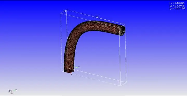
Elbow joint contains the throttle body over which we are interested to see the flow over the body.

Mesh

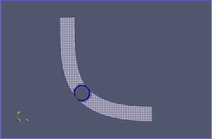
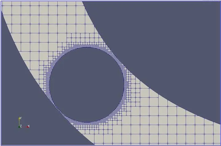
Figure shows the mesh structure developed by the cut cell cartesian method. Base size of 0.002m base grid was formed. As we can see near the holes, fixed embedding was employed to create a fine mesh around the body to study the flow parameters. Then we used the scale of 3 and added 2 layers of embedding to get this fine mesh.

SIMULATION TIME CALCULATION

From the steady state simulation it is observed that

Length of pipe = 0.2m

Average Velocity = 190 m/s

therefore we want to run the simulation for

Time = 0.2/190

Time = 0.001s

Since the cycle has to be repeated 10 times

Simulation end time = 0.001*10

Simulation end time = 0.01s

It is observed that we are going to run the simulation for 10 milli seconds.

BOUNDARY CONDITIONS

Inlet boundary

1. Inflow Boundary
2. Pressure = 1e5 bar
3. Mixture - air
4. Temperature = 300 K

Outlet Boundary

1. Outflow Boundary
2. Pressure = 1 bar
3. Mixture - Air
4. Temperature = 300 K

Throttle

1. Wall Boundary
2. Wall Motion - Moving
3. Temperature = 300 K
4. Turbulent Kinetic Energy - zero normal gradient
5. Turbulent Dissipation - Wall Motion
6. Turbulent Model - RNG K-Epsilon

Elbow Wall

1. Wall Boundary
2. Wall Motion - Stationary
3. Temperature = 300 K
4. Turbulent Kinetic Energy - zero normal gradient
5. Turbulent Dissipation - Wall Motion
6. Turbulent Model - RNG K-Epsilon

Results

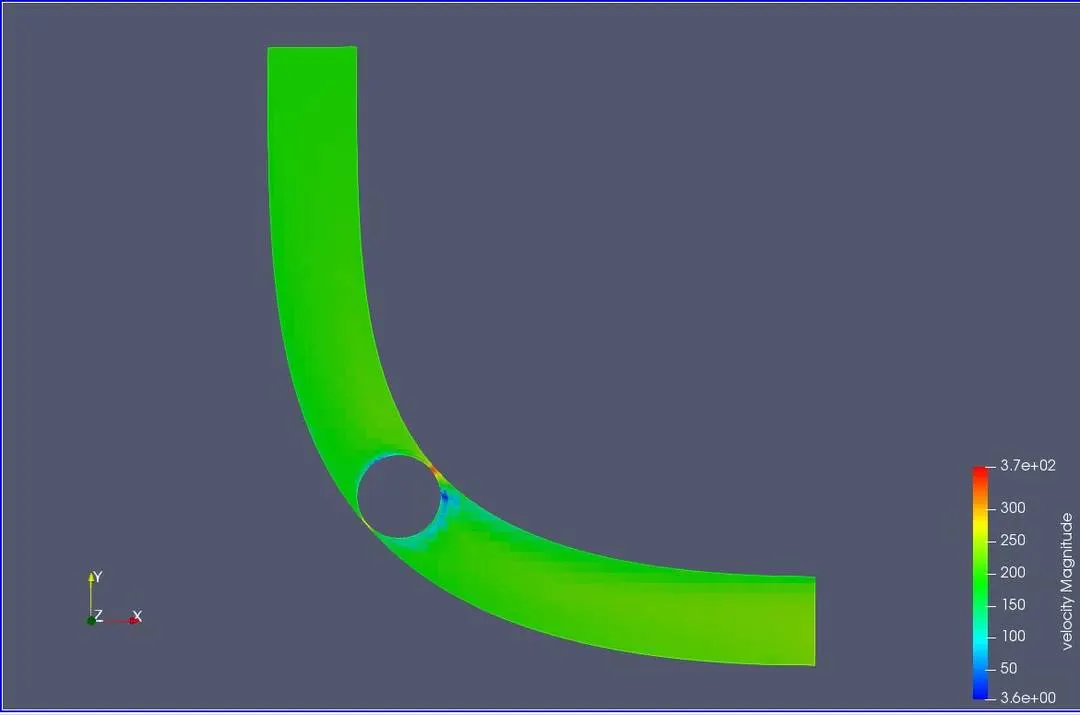
Velocity Contour

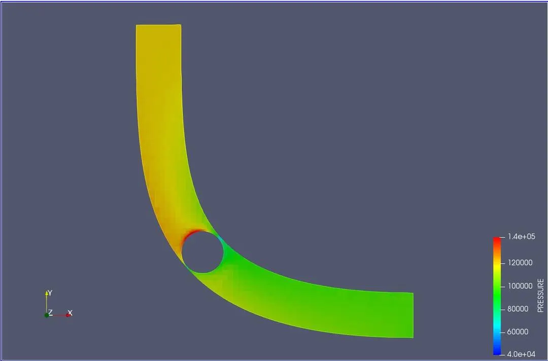
Pressure contour

Mass flow rate versus seconds

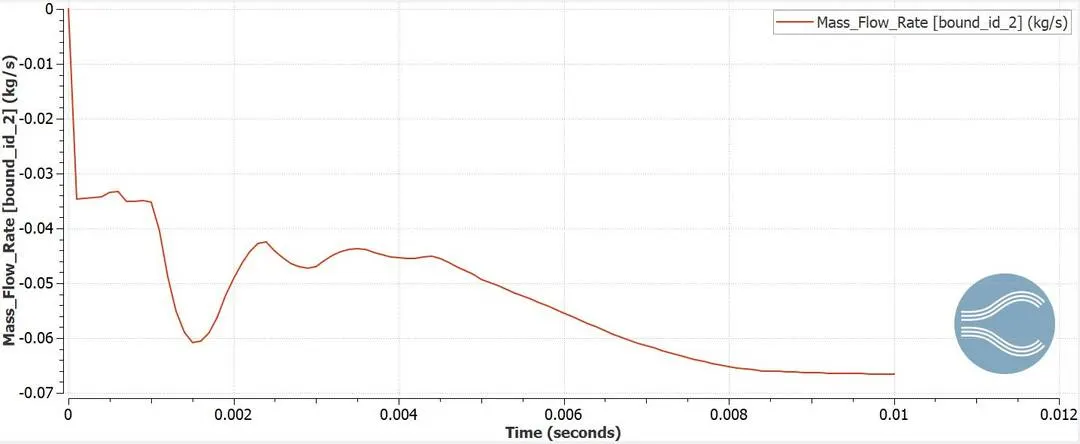
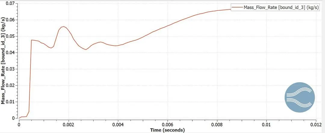
Now the mass flow rate says a value of 0.065 kg/s, which is the steady state value. Opposite signs in the inlet and the outlet plot means the mass is conserved which means the amount of air flowing through the inlet is almost same as the mass of air flowing through the outlet boundary.

Pressure versus seconds

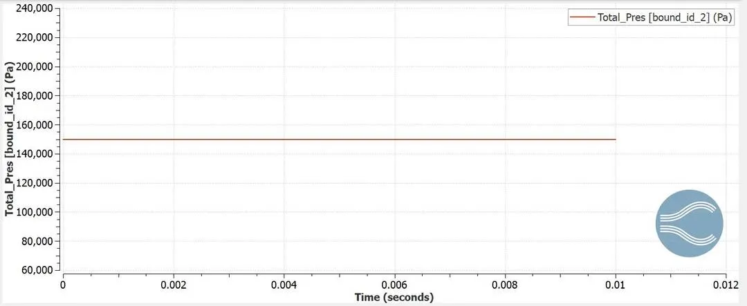
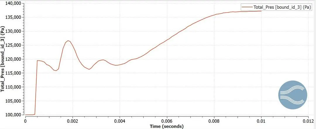
From the pressure plots we can see there is loss of pressure energy as the air flows over the throttle body. The inlet pressure is 1.5 bar and the outlet pressure is reduced to 1.35 bar showing pressure drop which occurs due to the flow

Velocity versus seconds

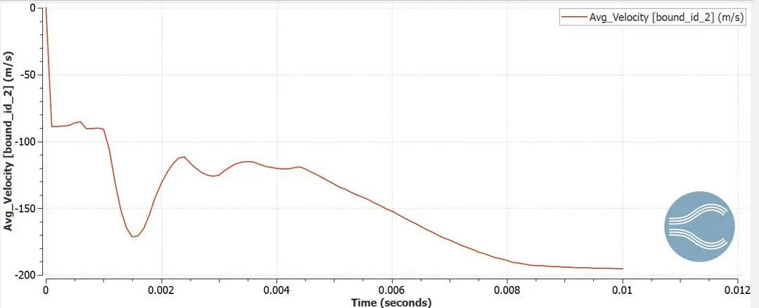
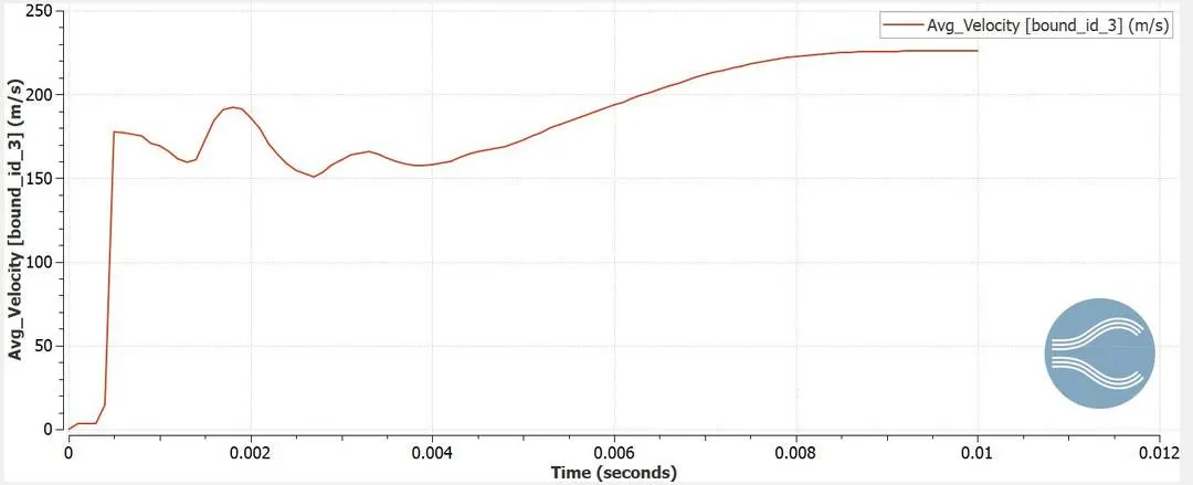
Inlet velocity has a value of 190 m/s but the outlet velocity has increases to somewhere around 230 m/s. This increase in the velocity is due to change in the pressure when the air flows over the throttle body keeping the area of cross section constant.

Cell count

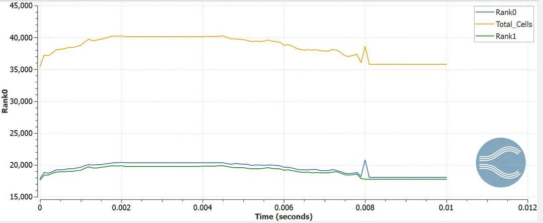
There are approximately 36000 cells that was generated during this simulation. This simulation was run in parallel with 2 processors with one having 17000 cells and the other processor takes 19000 cells to solve the governing equations of fluid flow.

THROTTLE BODY ANIMATION

CONCLUSION

1. The simulation of transcient flow over a throttle plate was run
2. Flow variables were analysed using paraview and converge line plot modules
3. The fundamental laws of fluid flow are conserved.