Week 4: Project - Transient simulation of flow over a throttle body

Aim:

To Setup and run transient state simulation for flow over a throttle body.

Objectives:

• To Post process the results and show pressure and velocity contours.
• To Show the mesh (i.e surface with edges)
• To Show the plots for pressure, velocity, mass flow rate and total cell count.
• To show the calculations on how you calculated an end time for the simulation.
• To Create an animation in which it throttle movement should be visible.

Procedure:

Step:1

Import given geomentry And modify the geomentry suitable for smulation.

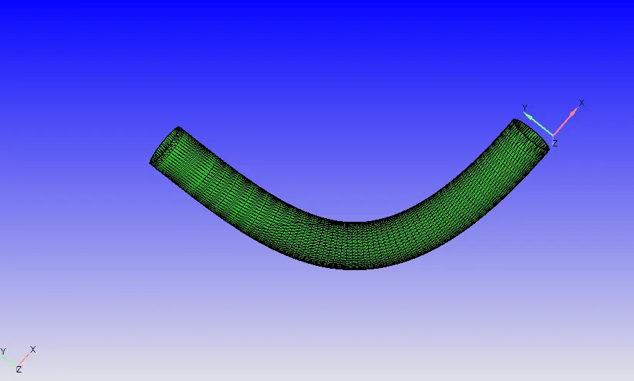
By using the boundary fence option The outer layer is removed .

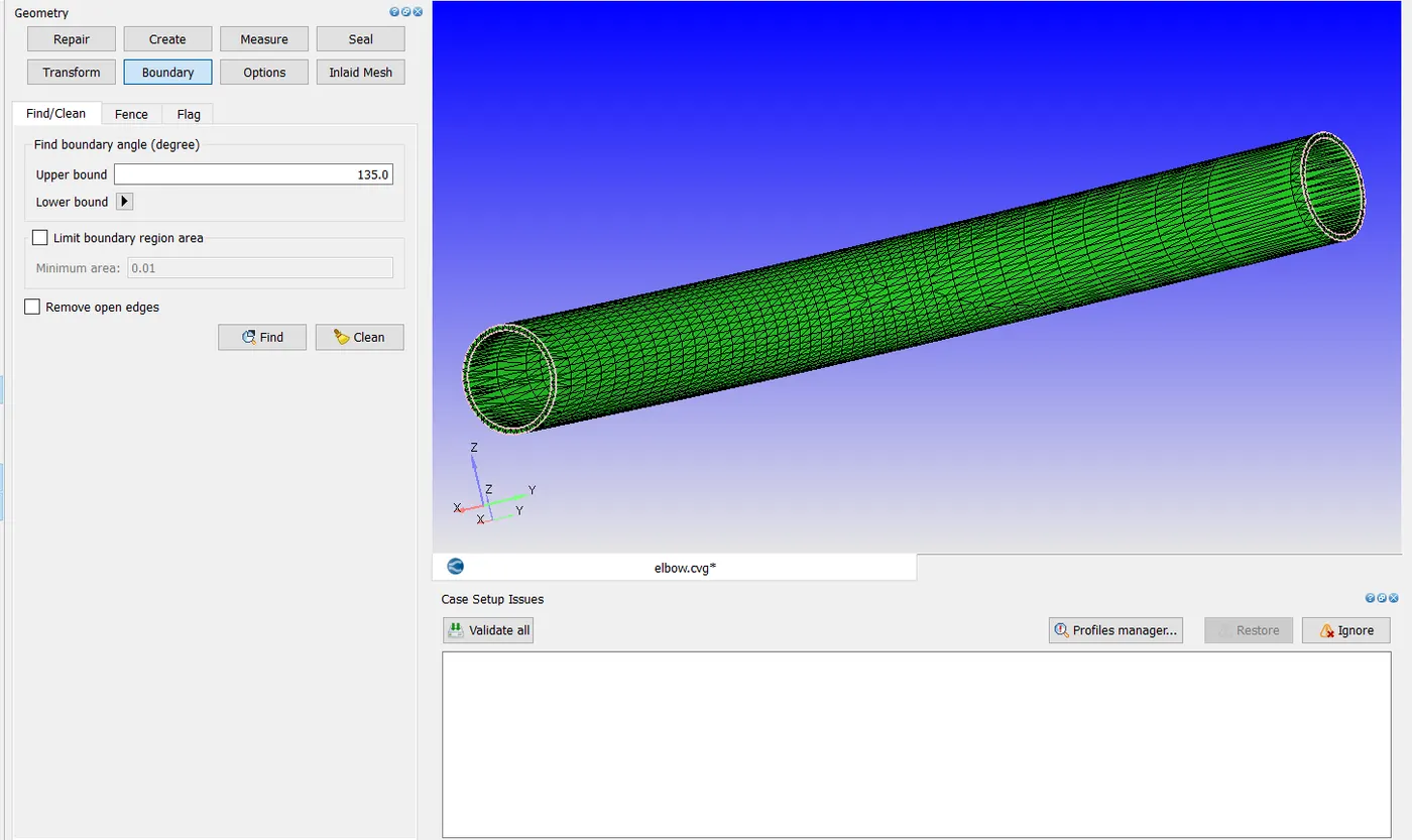
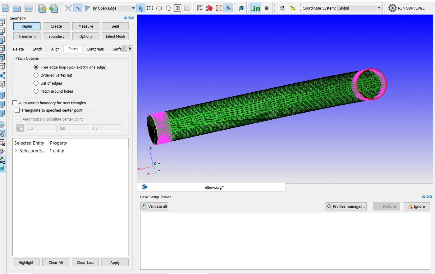
so that the free edges are poped and then it is rectified as using patch command.

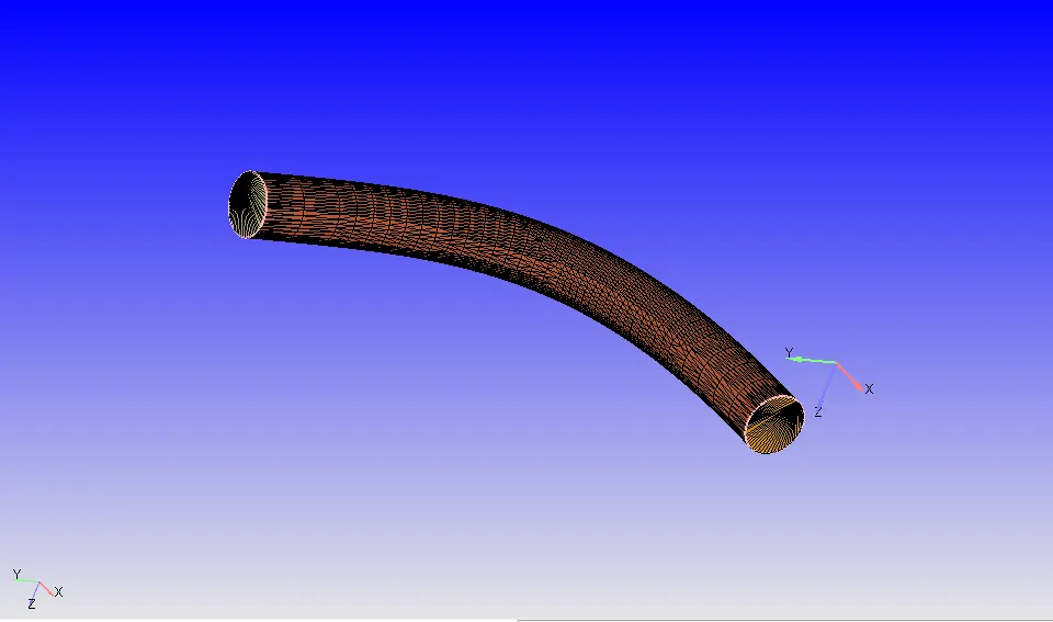
This is the final geomentry ready for simulation.

Step:2:

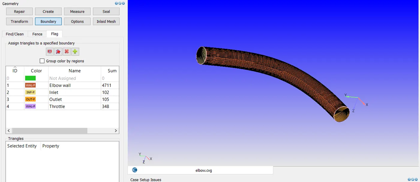
In this step, flag them together as boundaries which are marked with different colours.

Giving boundaries by selecting the sides which can help with other steps for simulation.

Once the boundaries have been flagged, we assign the different boundary conditions for the flow to take place within the geometry.

Step:3:

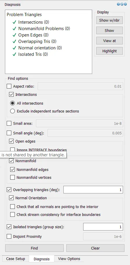
Check whether there is any errors by using diagnosis tool as shown below.

Step:4:

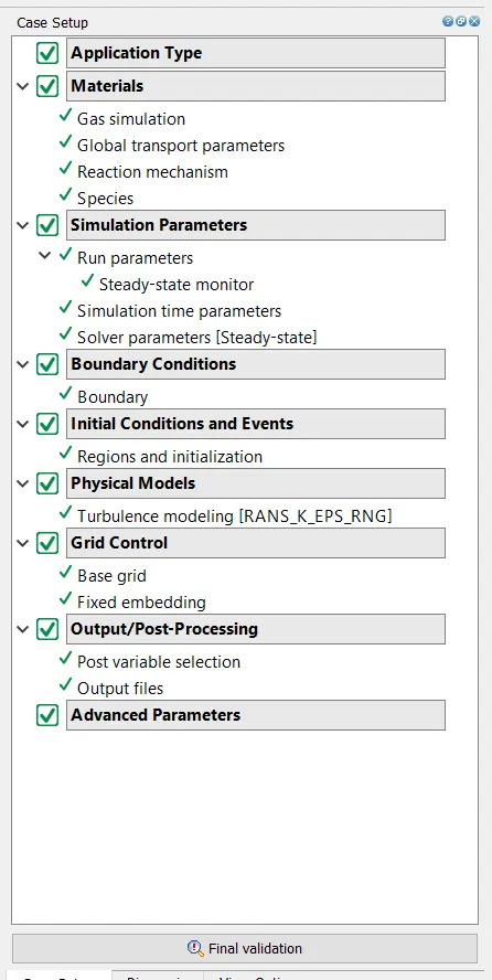
These are the following steps for setting up simulation .

Step:5:

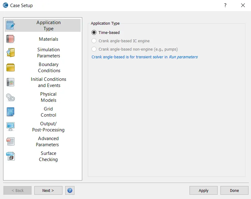
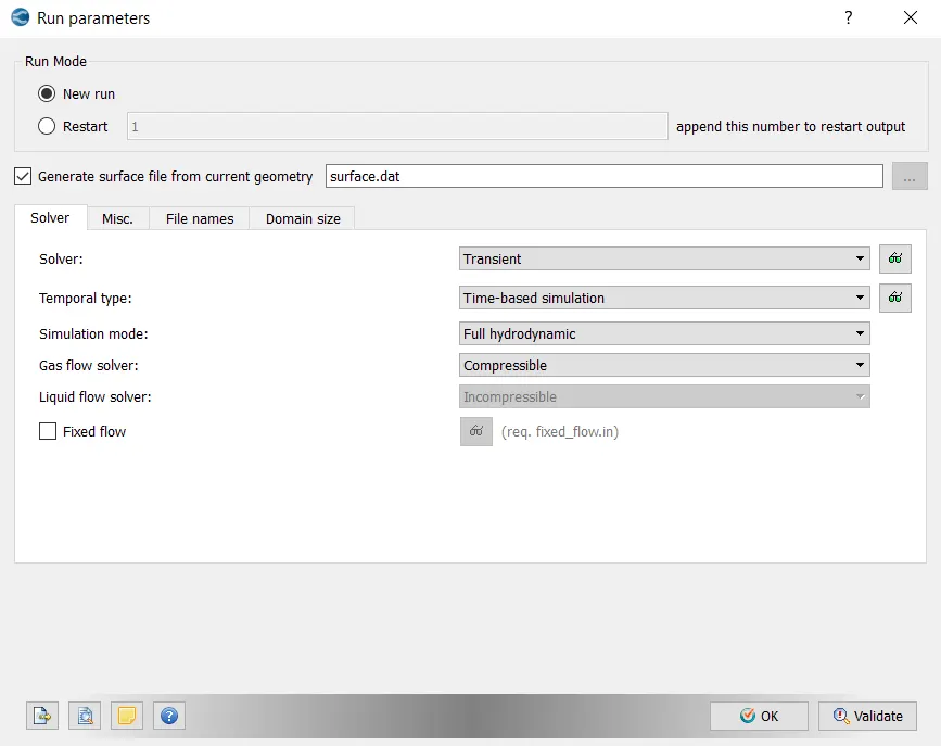
Select the application type time based for steady state simulation.

Step:6:

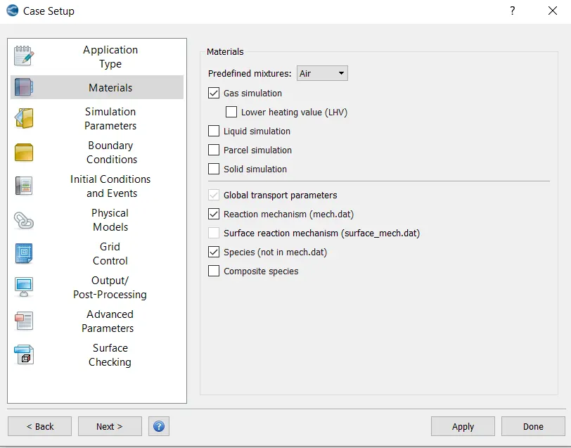
Select the material type for the flow through geomentry .here Air is the material taken.

Step:7

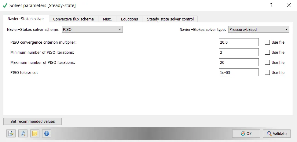
Select steady state solver for the simulation.and also pressure based

Step:8

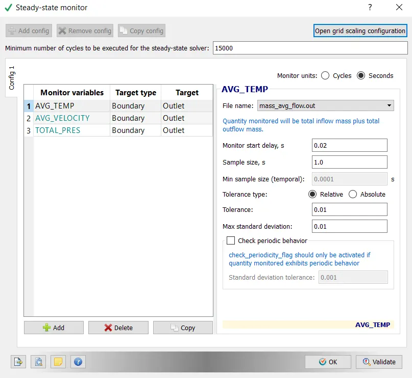
In Steady state monitor we can give minimum number of cycles for simulation .

Step:9:

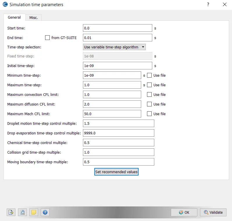
Here we can define the start and end time for simulation

and also the initial and minimum time step.

Here the throttle is moving so we define end time in seconds.

The calculation of end time is as follows.

End time = characteristic length / velocity

= 0.2 /191

=0.00104

End time = 0.00104* 10= 0.01 s(approx)

Step:10:

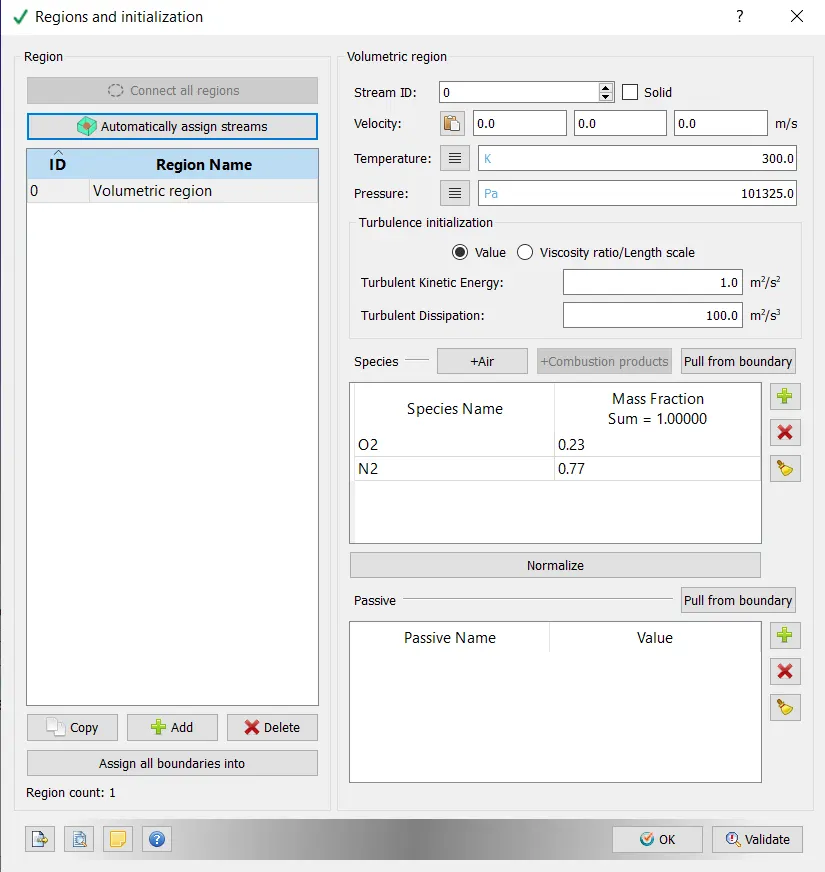
The boundaries are to bounded to a region for the steady simulation.so that volumetric region are created with the species of air.

Step:11:

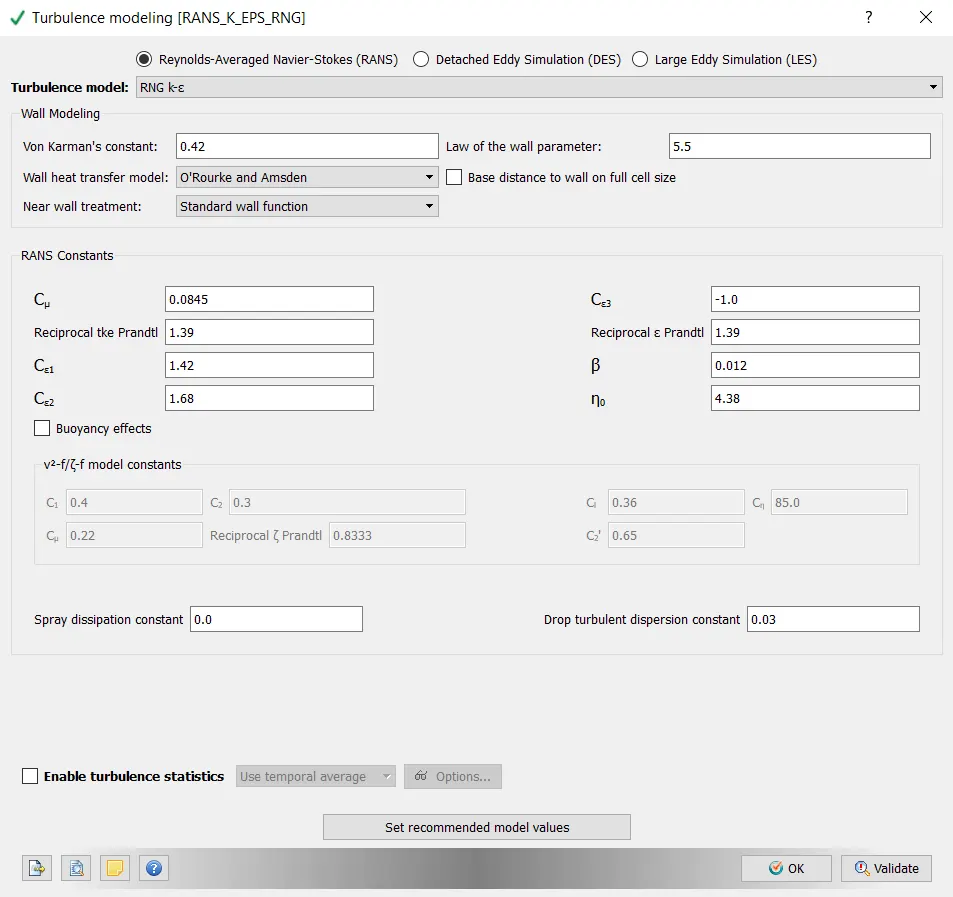
Here select the turbulance model that can be used for simulation.

Step:12:

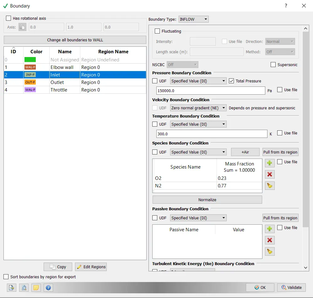
In here the boundary conditions are Assinged to the regions and also the inlet conditions are given .

pressure and temperature are defined for inlet.

Inlet:

elbow:

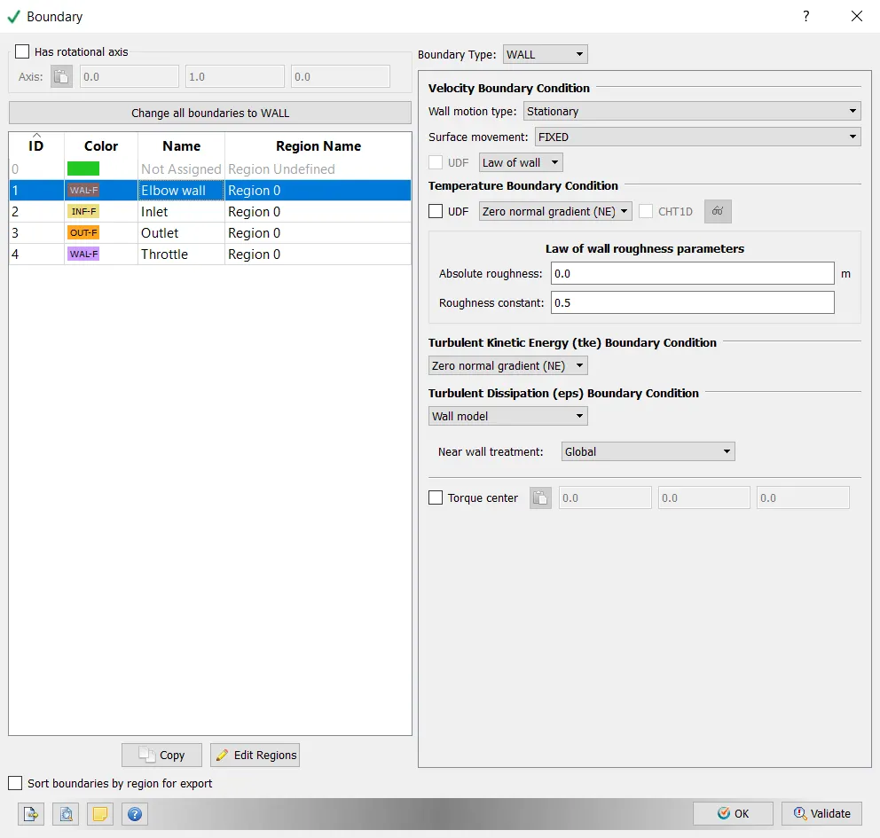
In here walls are defined to law of wall and temperature value is defined.

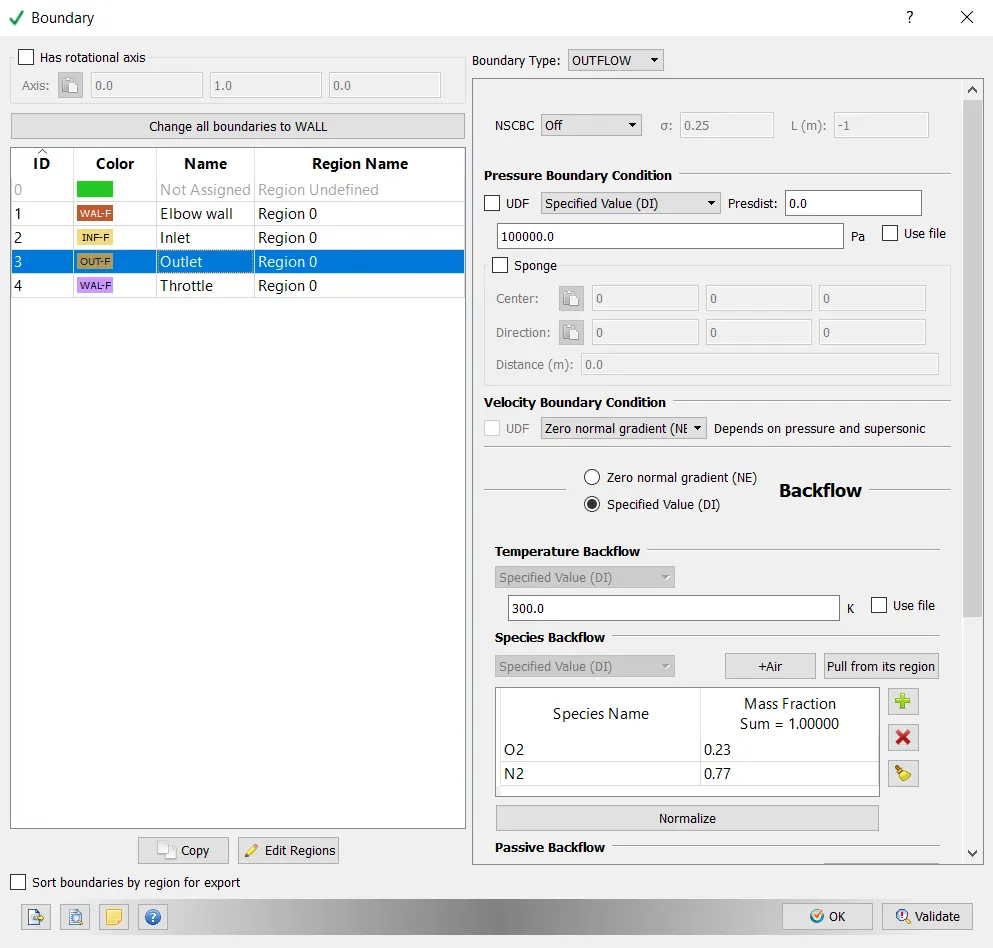
Outlet:

here the outlet pressure and temperature is given as specified value.

species used for simulation is defined in outlet.

Throttle:

Throttle motion is rotating and surface is moving type.

so we have to specify the rotation rate , rotation center and rotation normal.

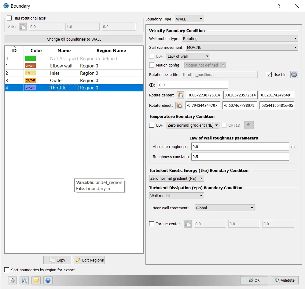
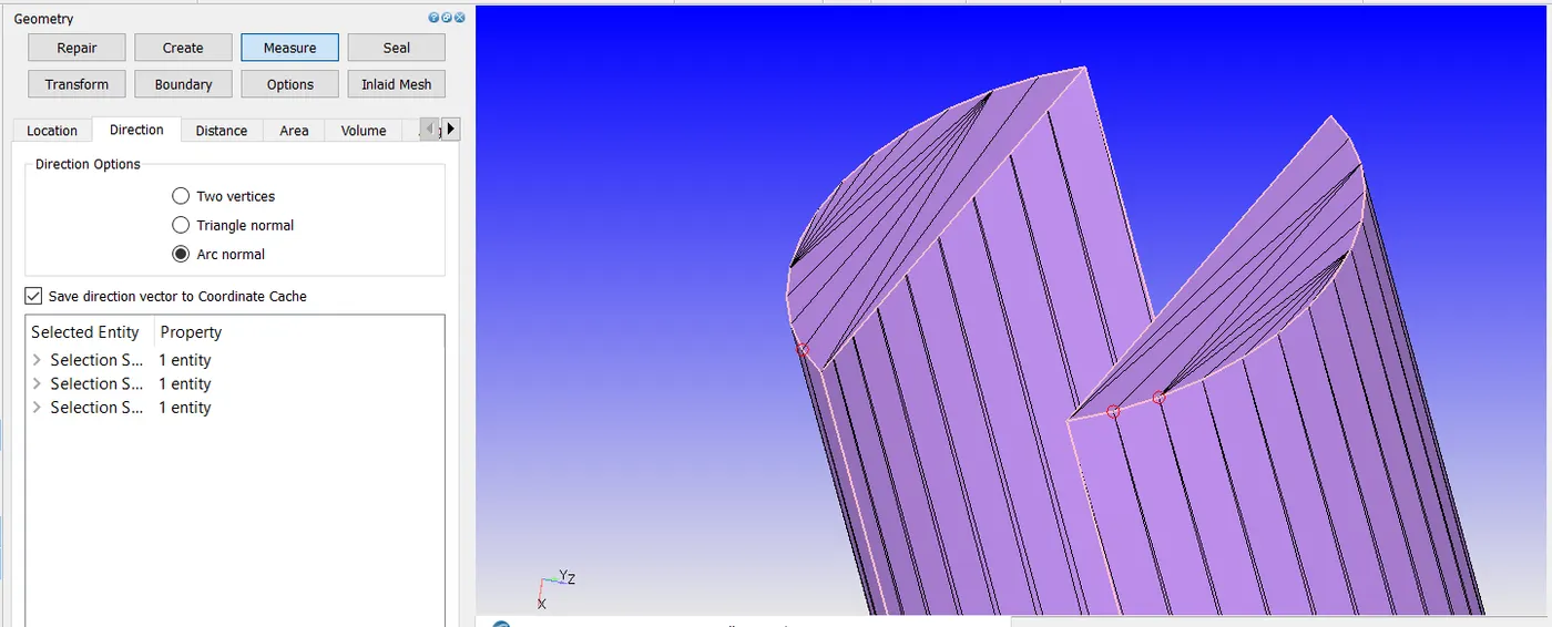
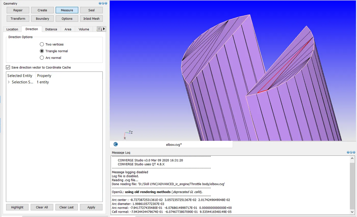
Here rotation center and rotate about axis is specifoed by using measure command in converge.

by measuring Arc normal with three points.

and also by selecting triangle normal as shown figures below.

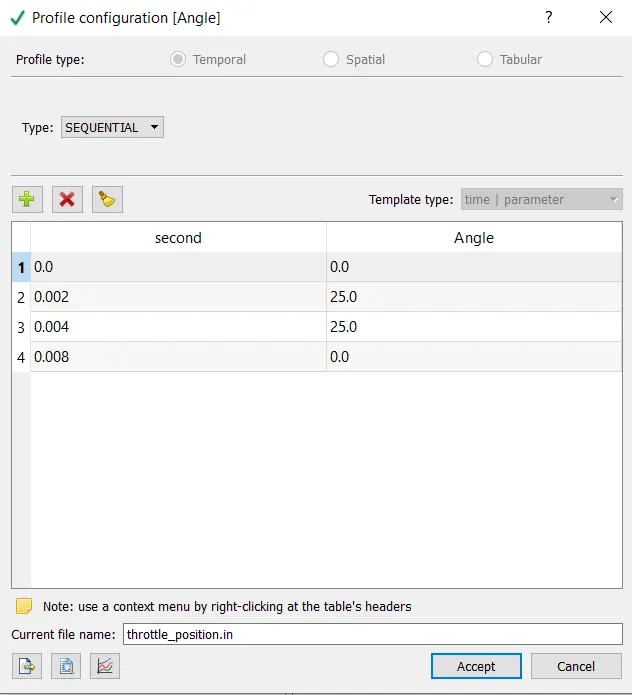
rotation rate file

The angle and the second which the throttle rotate and back to normal position is created in this file.

Step:13:

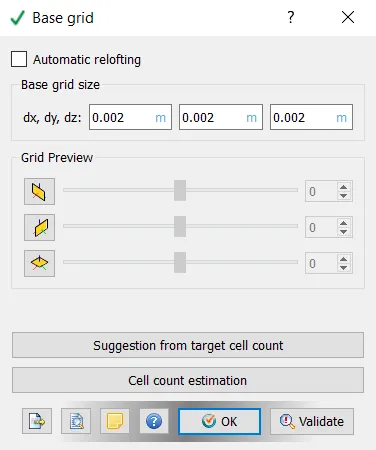
The basic mesh size of the Geomentry is specified here.

Step:14:

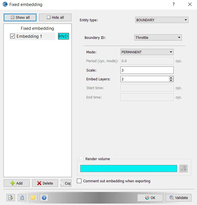
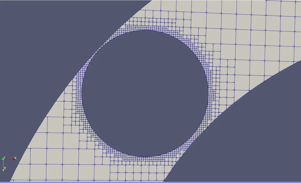
Here the mesh scale for Throttle are specified as below.

It is used to refine the mesh for desired regions.

fixed embedding = (base grid size)/2^n

grid size = 0.002 m

n = scale =3

embeded layer=2

Therefore fixed embeding = 0.002 /2^3

=0.00025 m cell size is present for 2 layer after that the base mesh size is present.

Step:15:

In output files the time interval for writing output data is specified in seconds.

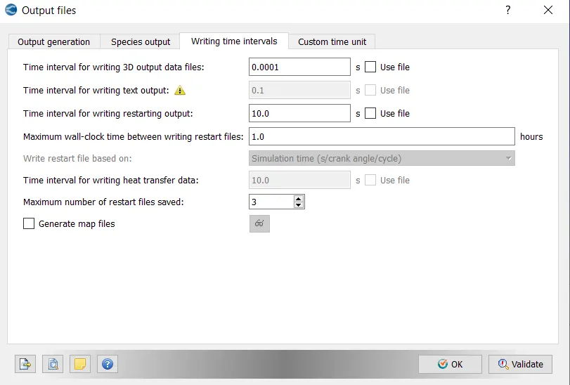
Finally the specified case setup file are exported to folder and run simulation.

The simulation for number of cycles are run in cygwin command window.

Step:16:

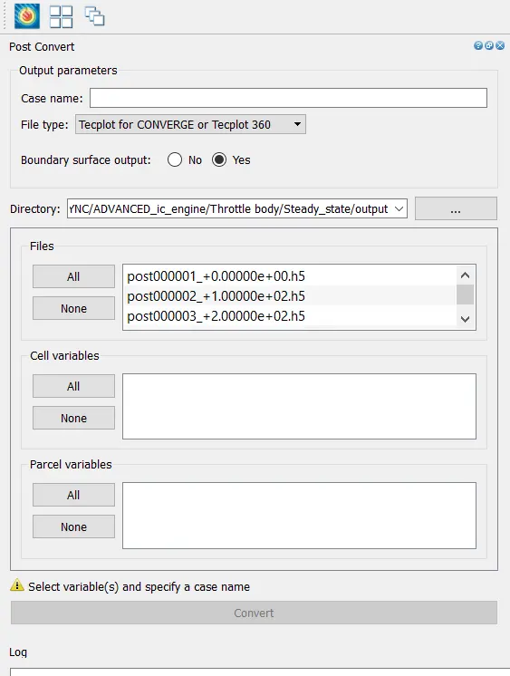
Post convert the files that is simulated in cygwin command window and file name is given .

Step:17:

Software used: ParaView As the simulation is binary files called “post” files are generated inside the output folder. These files have an extension *.out. Now these files are written by CONVERGE. These files contain information regarding the 3D flow field. We use a special software called ParaView that can read this flow information. However, before ParaView can do this, the files have to be converted to a form that ParaView can understand. This is done using a tool called post convert. After the conversion, we load the files into ParaView.

Results:

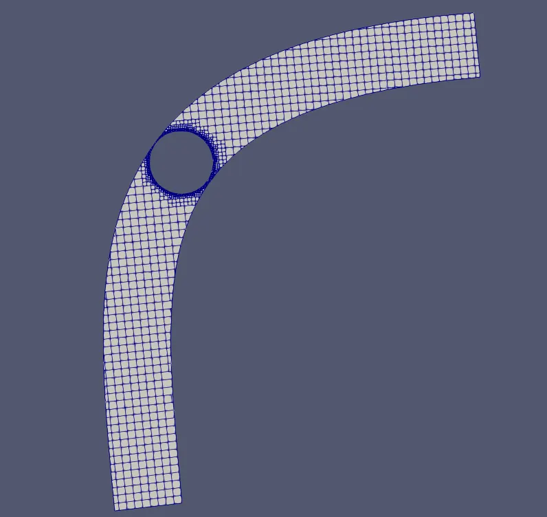
Mesh:

Animation Of mesh cells with throttle movement:

Contours:

Velocity :

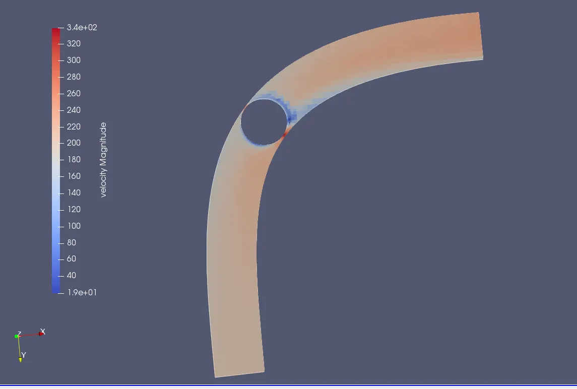
As the flow Approches the throttle body it encounters a narrow opening between the elbow and throttle . the lowest velocity is absorbed behind the throttle as its abstruct the flow.

Pressure:

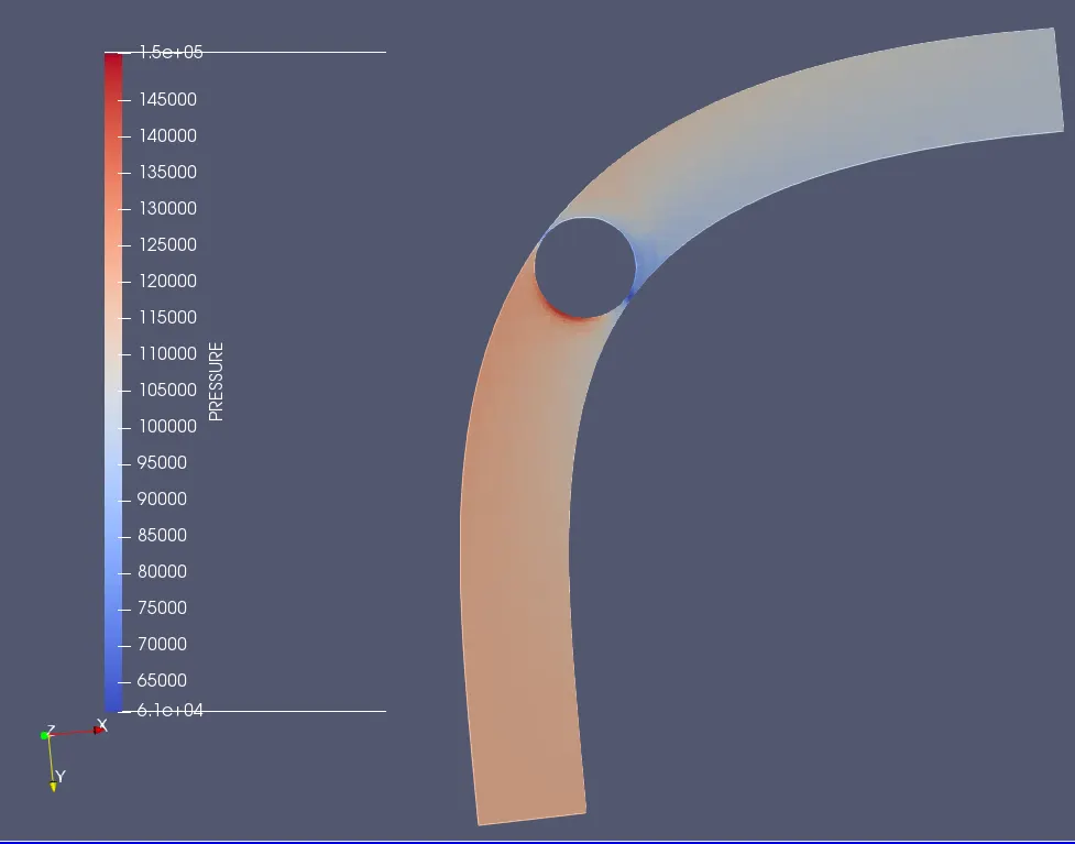
In here the pressure is highest in front of throttle body and lowest in narrow opening where velocity is highest.

Plots:

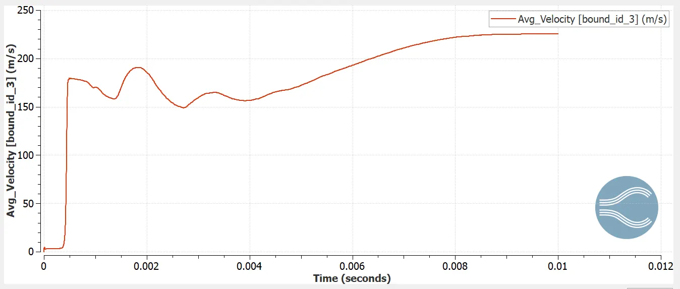
Velocity:

In velocity plot the outlet velocity is higher because of reduction of total pressure at outlet.

Pressure:

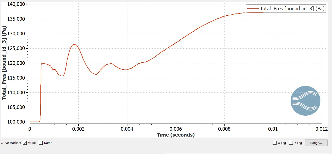
In pressure plot the outlet pressure decreases which means the outlet velocity is increases. this is due to the air passes from small cross-section area velocity increases and pressure decreases.

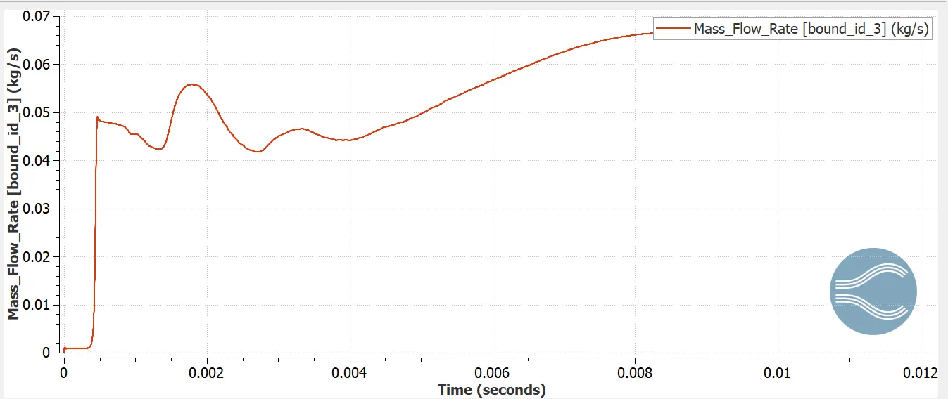
Mass flow rate:

For steady state simulation it is important to check convergence has attained. so from mass flow rate The convergence of outlet flow has been covered.

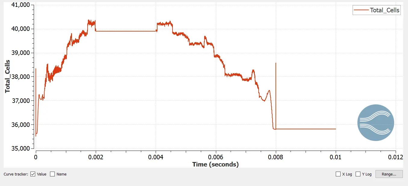
Total cells:

The number of cells is varying due to movement of throttle.

Animation:

In animation vedio of The movement of throttle is clearly obsorbed.

The velocity passes through the throttle how it is varying is shown in animation below.

Conclusion:

Here it is found that drastic increase in total cell count when the throttle body moves from o to 2ms and the cell remains constant for 2 to 4 ms as throttle remains constant and then cell count decreases as throttle body comes to original position as shown in mesh animation above.

As throttle body rotates there is obstriction in flow and hence it velocity and kinetic energy converted into pressure energy so that pressure increases.

velocity is initially zero, as throttle rotates to 25 deg maximum .then it attains steady state during dwell time of throttle so there is low velocity region formed right before and after throttle.

As throttle plate rotates to 25 degree the upstream gets pressurised.The region exactly before throttle is high pressure regions and the region after throttle is low pressurised.