Week 4: Project - Transient simulation of flow over a throttle body
Aim :
To Set-up and run a Transient simulation for the flow of air through an Elbow shaped pipe having a Throttle valve placed at the curve of the Elbow parallel to the direction of flow.
To Post process the results and show pressure, velocity contours, Meshing, plots for pressure, velocity, mass flow rate and total cell count.
Geometry & Introduction :
Download the Given .STL file and import the file into converge.
The given geometry consists of an elbow shaped pipe with two openings (Inlet, Outlet). A throttle valve is placed in between the pipe.
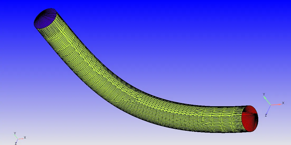
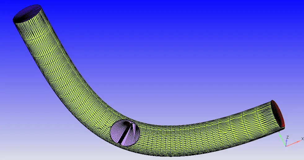
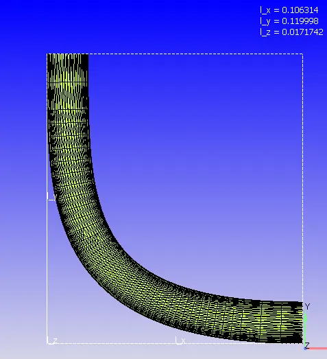
Now scale the whole geometry for a factor of 0.001 to convert the units to mm.
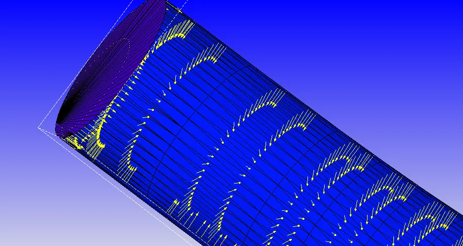
The flow is taking place within the pipe. Which means the normals should be pointed inside the geometry.
Now all the properties of the geometry are prepared and is ready to be simulated.
Let us assign some boundary namings to distinguish the parts of the geometry.
Consider one end of the pipe as Inlet and the other end as Outlet.
The outside wall of the pipe is named as elbow and the valve is named as Throttle.
Set up & Simulation :
Start the case set up by selecting the Time-Based Application.
Choose air as the material of flow through the pipe.
As we consider the throttle to be rotating inside the pipe we choose transient simulation.
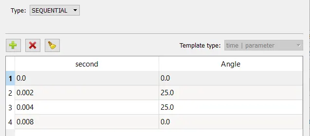
The rotation of the disc is considered to be done in the following steps:
- From 0 to 2 ms the valve should rotate by 25 degrees.
- From 2 to 4ms it should stay at 25 degrees.
- After which by 8ms the valve should get back to it’s original position.
Calculating Flow time :
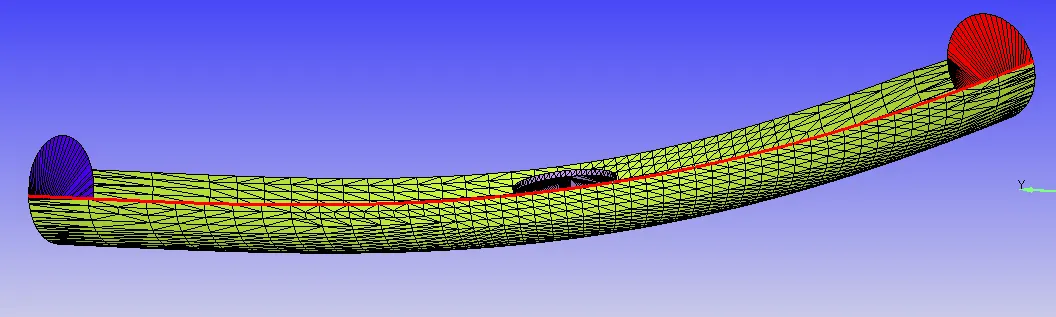
The total length of the pipe marked is 1.9063538209263E-01 m.
The average inlet velocity is 193 m/s.
By dividing the inlet velocity to the length of the pipe we can get the flow time to be 1 milli second (0.001 second).
As we are rotating the the disc at some time period, let us take the time taken foe the flow to be 10 milli seconds.
Give the end cycle time to be 0.01 seconds (10 milli seconds) with valid CFL values.
Boundary Conditions :
Inlet :
Boundary type : INFLOW
Pressure : 150000 pa
Temperature : 300 k
Species : Air
O2 mass fraction : 0.23
N2 mass fraction : 0.77
Outlet :
Boundary type : OUTFLOW
Pressure : 100000 pa
Temperature : 300 k
Species : Air
O2 mass fraction : 0.23
N2 mass fraction : 0.77
Elbow : Wall
Throttle : Wall
To give the coordinates for the rotate center and the axis let us measure the coordinates of the throttle cylinder.
Go to measure in the geometry tree and go to direction and using the option arc normal we can find the center and axis of the arc of the cylinder.

Give the coordinates in the boundary conditions.
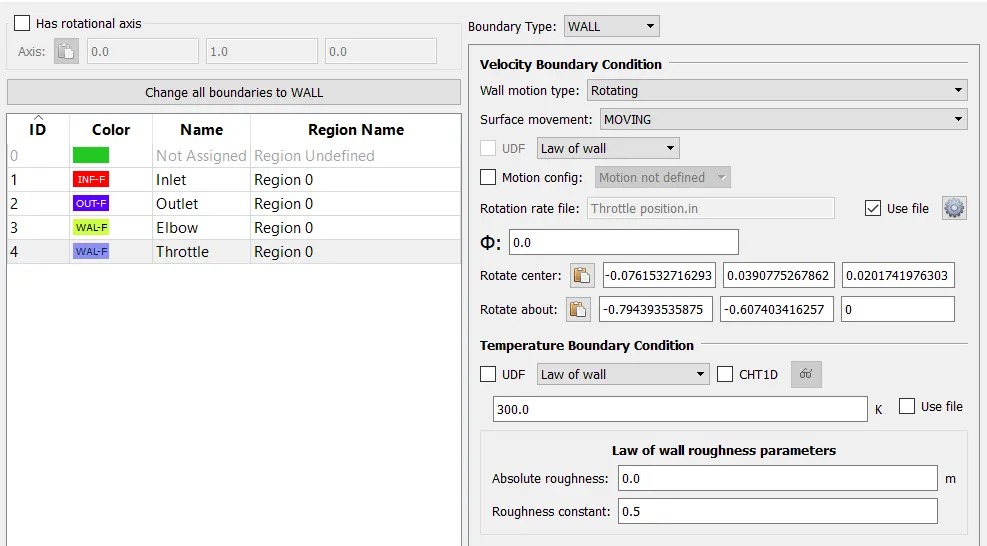
To provide the timings of the disc opening and angle, use a file.
Assign the conditions to a region with species Air and Default conditions.
Use K-Epsilon Turbulence model for the simulation.
Base Grid :
The overall grid size is taken to be 0.002 m.
Still we have very small gaps between the throttle and the elbow wall.
Fixed Embedding :
To refine that critical area, we can use Fixed Embedding around the Throttle Boundary.
fixed embedding is used to refine the grid at specific locations in the domain where a finer resolution is critical to the accuracy of the solution. Fixed embedding allows the rest of the grid to remain coarse to minimize simulation time.
For each fixed embedding, you must specify an embedding scale that indicates how CONVERGE will refine the grid in that location. The embed_scale parameter, which must be a positive integer, scales the base grid sizes (dx_base, dy_base, and dz_base) according to
dx_embed = dx_base/2^embed_scale.
Note that CONVERGE requires two-to-one connectivity between cells, i.e., a cell with an embed_scale of 2 can be adjacent only to a cell with an embed_scale of 1, 2, or 3. To maintain the required connectivity, CONVERGE provides cells with intermediate embed_scale values as necessary.
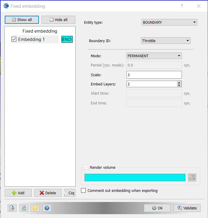
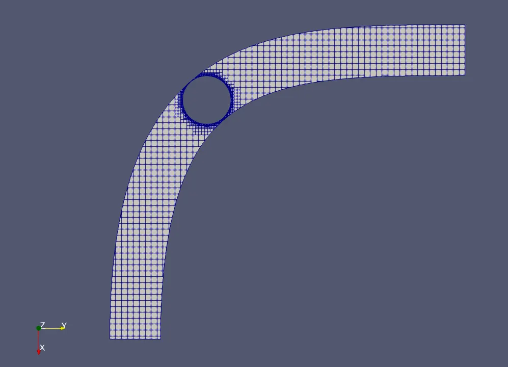
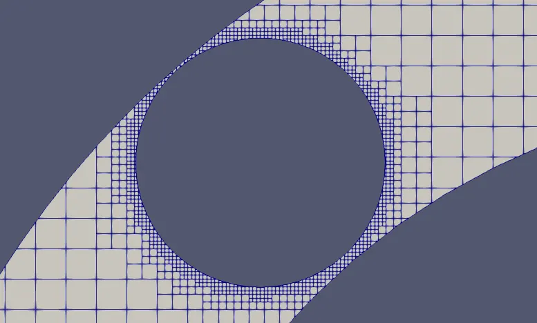
After Applying the mesh values we can find the area around the throttle to have finner meshing as you can see in the figure attached below.
As we have a rotating part inside the fluuid volume, the cutcells rearrange the cells around the moving part whenever there is a change i position.
Calculation :
According to the conditions specified in the casse setup, the input files can be exported to the folder.
Open cygwin to perform the calculations using the input files.
Use converge-intel.exe command to calculate the results.
Convert the output files into EnSight format using converge.
Post process the results using Paraview.
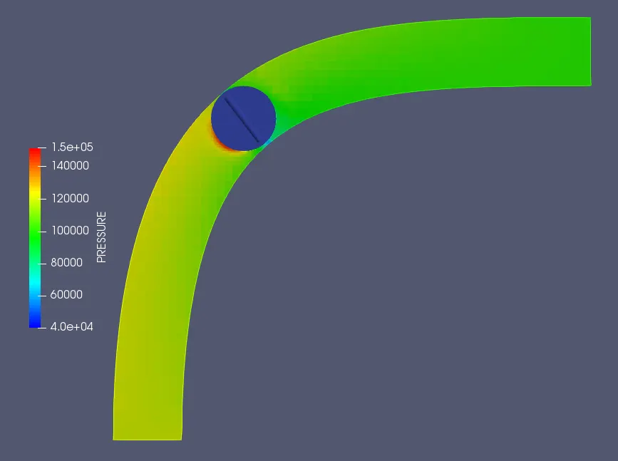
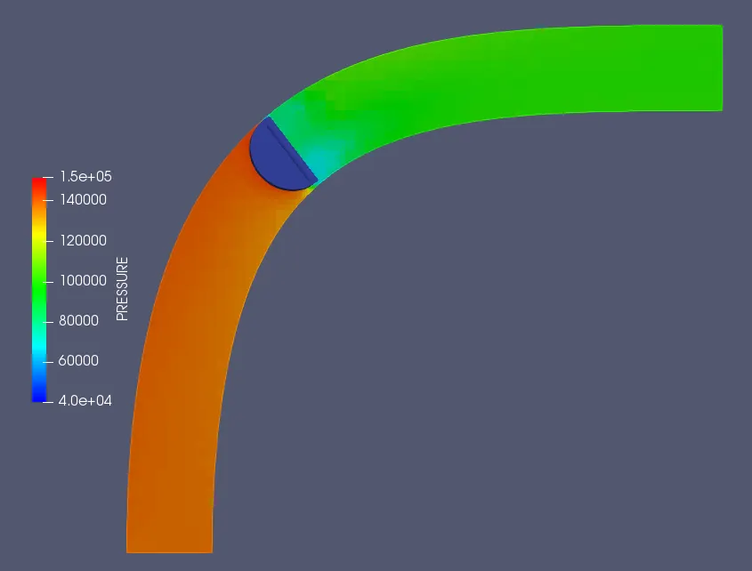
Pressure Contour :
0 degree : 25 Degree :
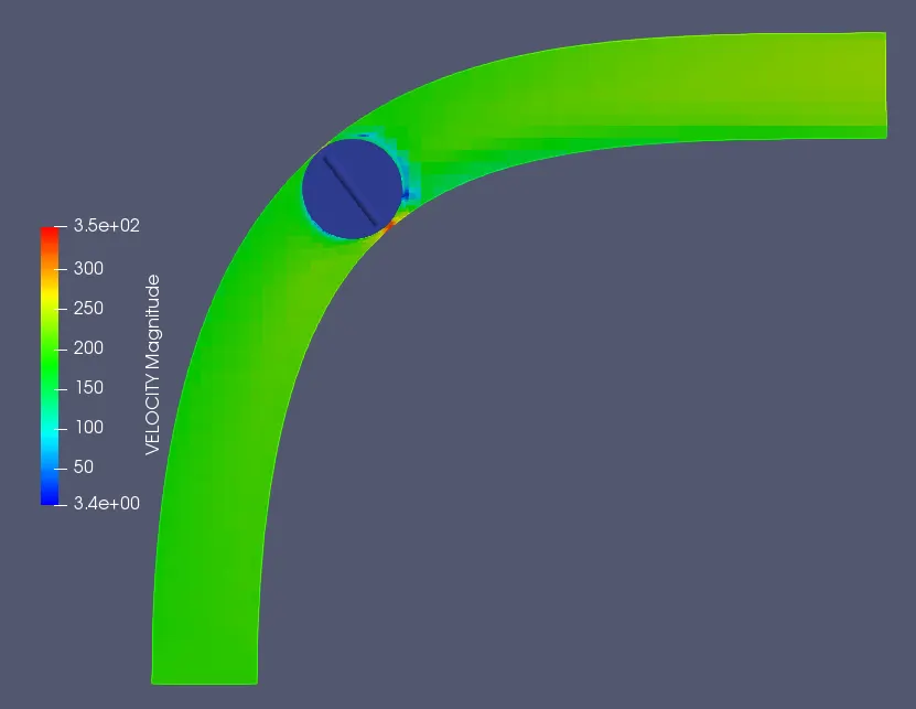
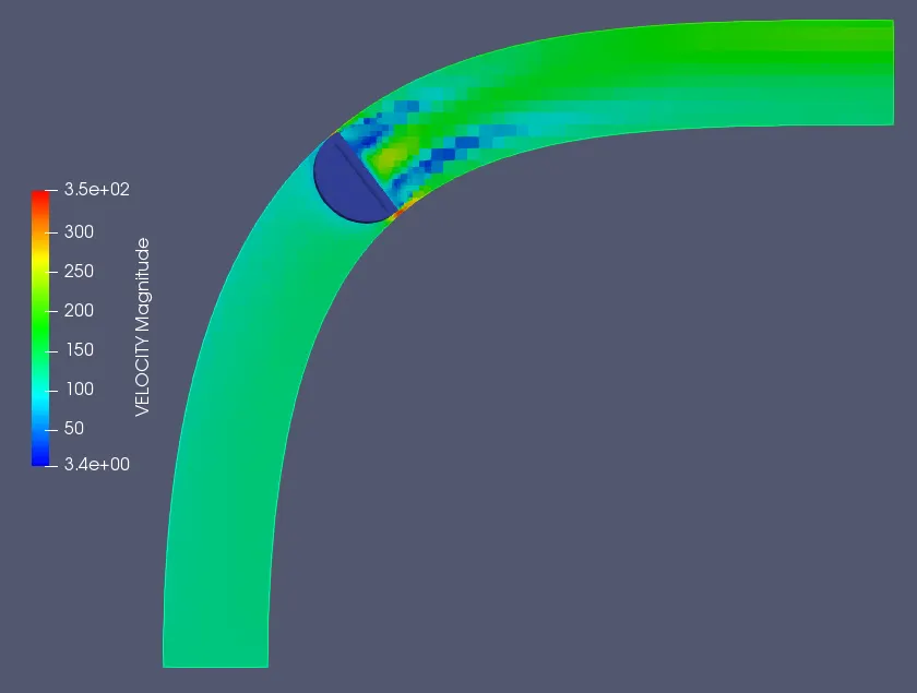
Velocity Contour :
0 degree : 25 Degree :
Streamline flow & Throttle movement :
Conclusion on contours :
In the velocity contour, we can see that the velocity is maximum at the gap between throttle and the pipe wall when the valve disc is fully open (0 Degree).
As the valve disc rotates 25 degree, the velocity of the flow encounters a higher area of contact and thus loses its velocity gradually.
We can see that the velocity flow is minimum at the center axis of the disc.
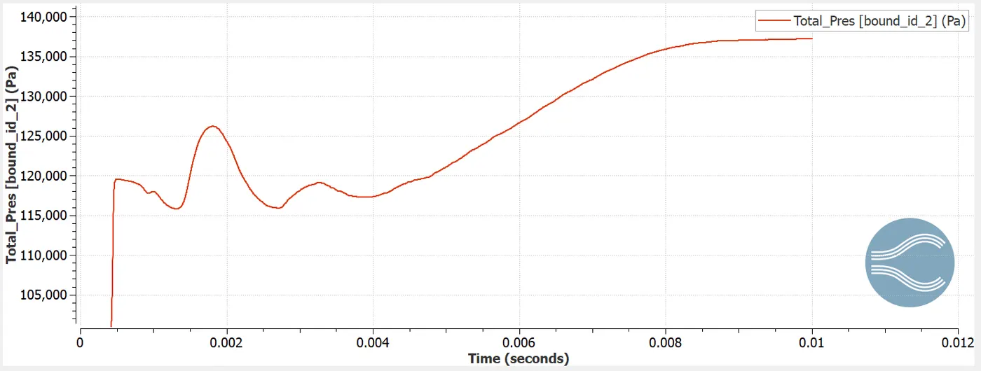
As the disc rotates we can see that the inlet pressure increases as the disc tends to reduce the volume of fluid flow. This causes a resistance towards the flow that damps the fluid to increase the pressure.
As soon as the disc rotates the flow tends to move around the disc causing some non-uniform motions around the valve disc.
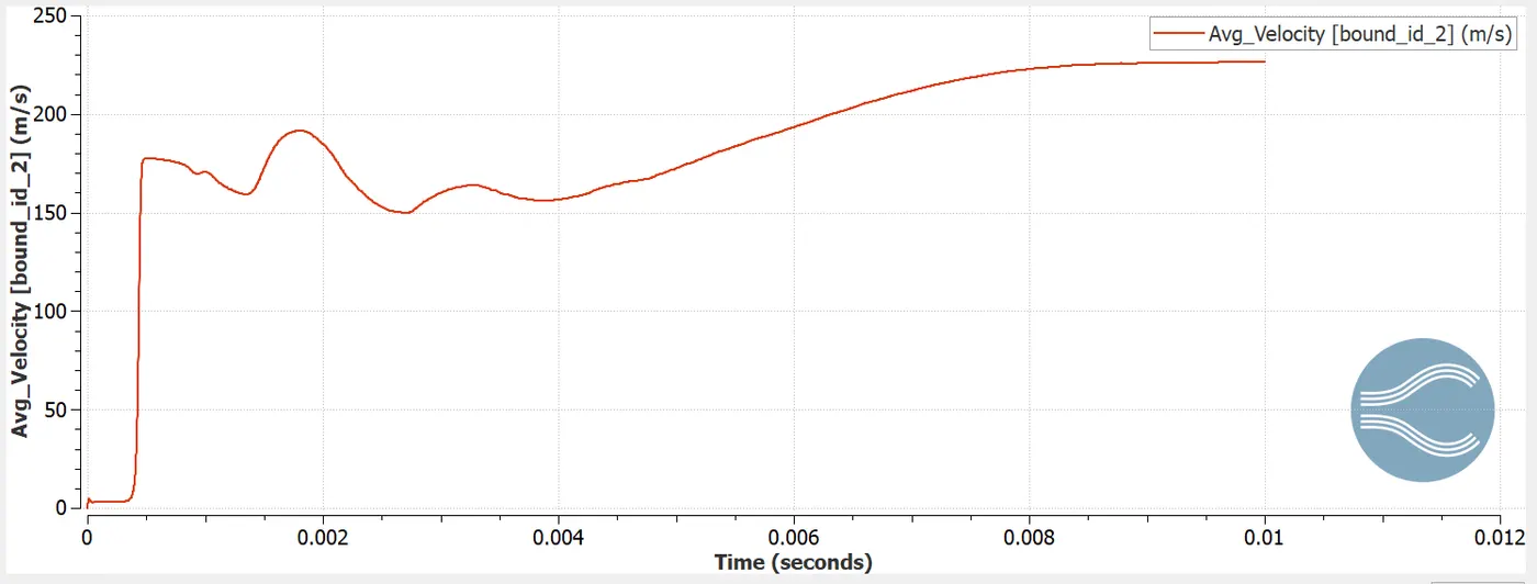
Velocity plot at outlet :
Pressure plot at outlet :
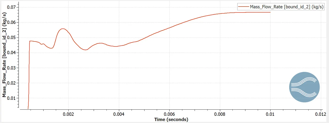
Mass Flow Rate plot at outlet :
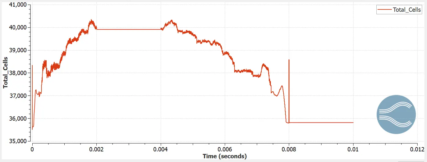
Total Cell Count :
Conclusion on Plots :
The cell count changes as the disc starts to rotate gradually to an angle of 25 degree. Then as the disc stays in the same position between 0.002 to 0.004 seconds the cell count stays constant during that period of time. Then the disc moves back to its original position changing the cell count which again gets constant as the disc attains the original position.
The velocity and mass flow rate of the flow decreases as the disc tends to close the pipe. Because of the decrease in the fluid volume the mass flow rate also decreases. Then as the disc gradually moves to its initial position, the velocity and mass flow rate gradually increases with the gradual increase in the fluid volume and finally after the disc is fully opened again, the flow attains convergence.