Steady state simulation of flow over a throttle body
Aim: To do steady state simulation for fluid flow over throttle body and discuss the results obtained.
Introduction:
The throttle valves are the devices that control the fluid flow by obstruction or constriction. The throttle valve is mainly used to monitor the fuel or air supply into the IC engine. Thus with the help of throttle valve the speed of the vehicle is controlled. In this project, the behaviour of the fluid when it is made to flow over the fixed throttle body (no movement or rotation) is studied. The steady state simlation for flow over throttle body is done with the help of converge cfd software. The case setup and results for the simulation is discussed below.
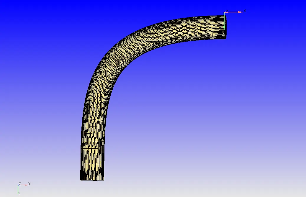
Geometry of the throttle valve:
Boundary conditions:
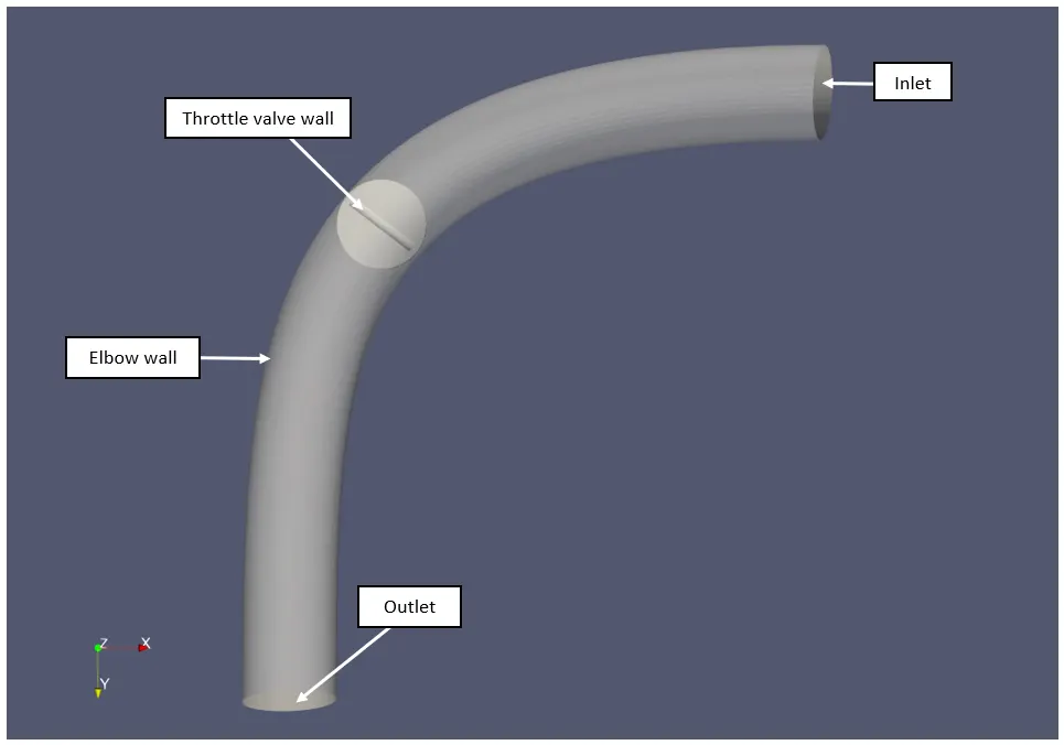
Inlet:
Boundary type = inlfow
Total pressure = 150 k pa
Temperature = 300k
Species = air
Outlet:
Boundary type = outflow
Static pressure = 100 k pa
Temperature = 300k
Species = air
Elbow wall:
Boundary type = wall
Wall motion type = stationary
Surface movement = fixed
throttle valve wall:
Boundary type = wall
Wall motion type = stationary
Surface movement = fixed
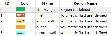
Assigning volumetric fluid region to all the boundaries
Resion name = voumetric fluid used defined
Species = air
Pressure = 101325 pa
Temperature = 300k
Solver type = Steady state pressure based solver
Solver scheme = PISO
Simulation parameters:
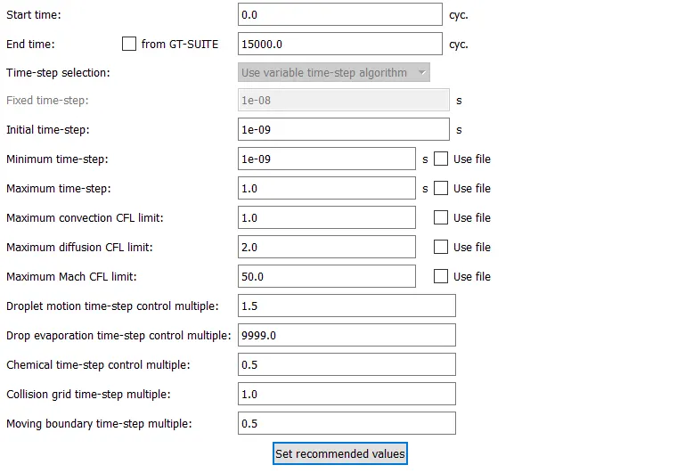
The given throttle body model is imported into the converge CFD software. The boundary conditions are flagged to all the respective regions and the air is added as the fluid medium into the volumetric region. The total pressure at inlet 150 k pascals and static pressure at outlet is 100 k pascals, due to this pressure difference the fluid steam flows from the inlet to the outlet. Steady state pressure based solver is used to solve the problem as the throttle valve is fixed or stationary and fluid flow around the throttle valve is to be observed. The PISO solver scheme (pressure implicit with splitting of operator) is prefered as this scheme gives accurate results and good wall treatment is done and gives stable solution.
Mesh generated
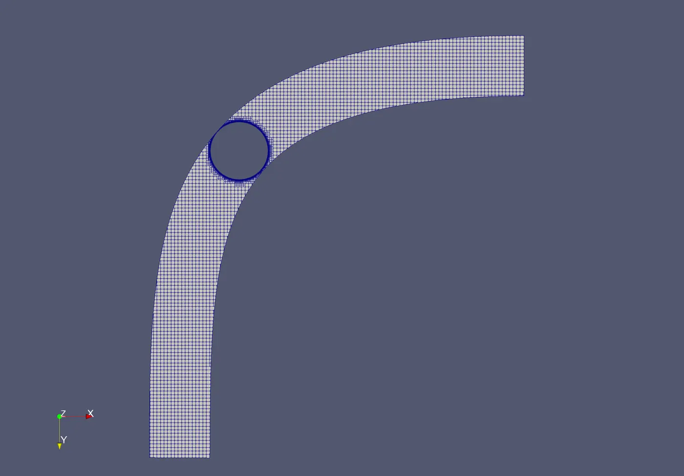
Base grid size: dx=dy=dz= 0.002 m
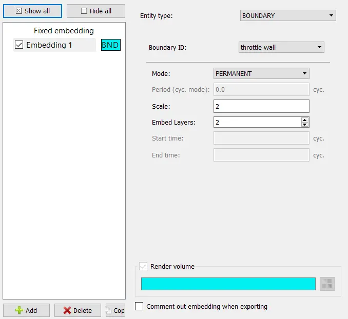
Fixed embedding
Total cell count
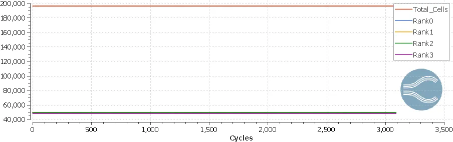
The above figure shows the mesh generated with base grid size equal to 0.002 m. The embedding layers of two is generated near the throttle valve ti capture the fluid behaviour near the throttle valve wall. From the total cell count plot it can be seen that 200k cells is generated (more the number of cells accurate the results).
Results:
Velocity contour
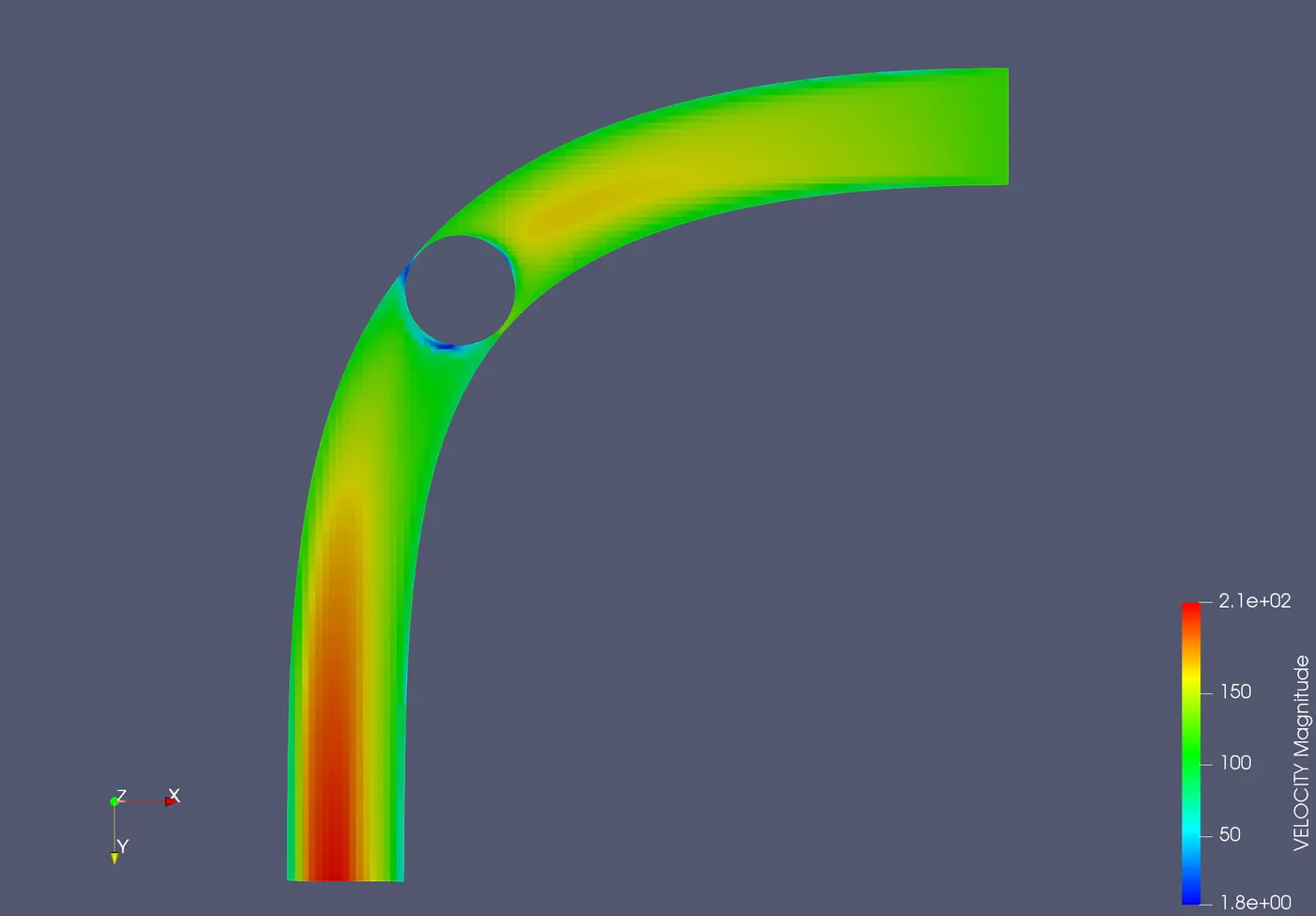
Velocity vector plot
Velocity animation
Pressure contour
Density contour
Velocity plot
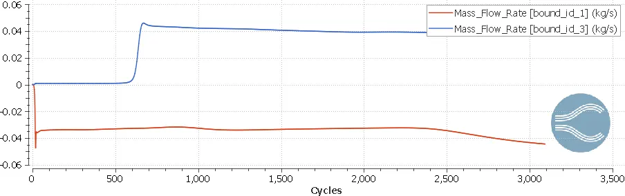
Mass flow rate plot
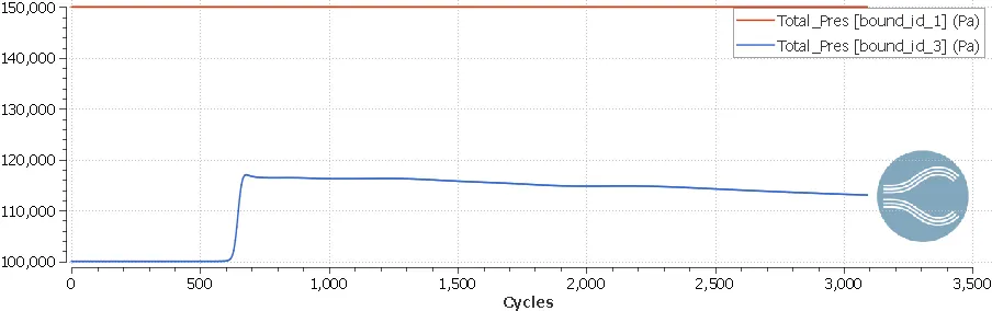
Total pressure plot
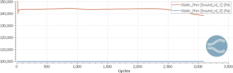
Static pressure plot
Conclusion:
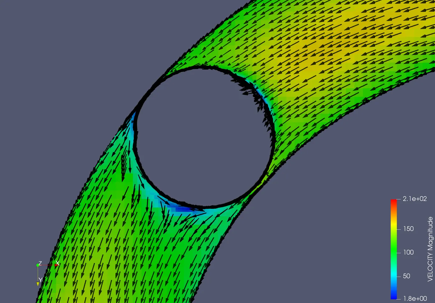
- In the velocity contour, it can be seen that the velocity of the fluid reachs zero near the throttle valve due to obstruction. This point where the fluid velocity reaches zero is called as the stagnation point. As the fluid passes through the throttle valve, the velocity of the fluid increases.
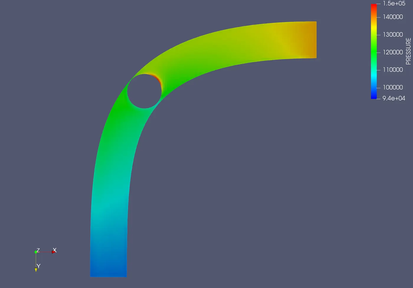
- In the pressure contour, it can be seen that the fluid experiences high pressure of 1.5e5 pa near the walls of the throttle valve, this is because the fluid velocity is zero near the throttle valve walls.
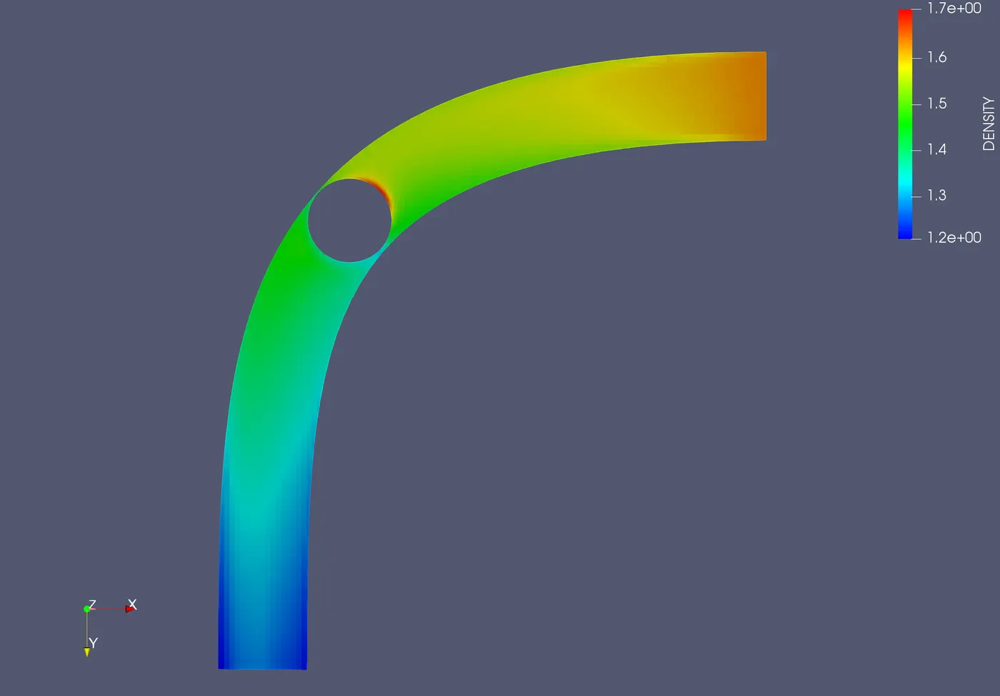
- In the density contour, the density of the fluid changes from 1.2 to 1.7 as it passes through the throttle valve this is due to increase in pressure across the throttle valve.
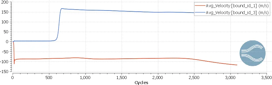
- In the velocity plot, it can be seen that fluid velocity increases as it flows from inlet to outlet. This is due to increase in the flow area.
- In the mass flow rate plot, both flow rates at inlet and exit is same hence the flow is continuous. And the plot shows both positive and negative values which implies that mass is conserved.
- In the total pressure plot, it can be seen that the total pressure is constant at inlet due to boundary conditions and increases at outlet due the increase in fluid velocity which further increases dynamic pressure.
- In the static pressure plot, it can be seen that the static pressure decreases at inlet due to increase in fluid velocity and static pressure remains constant at outlet due to boundary conditions.