Week 4 - Genetic Algorithm

Objective

1. To expalin the concept of genetic algorithm
2. To optimise the stalagmite function and find the global maxima of the function. Plot graphs for all 3 studies and for F maximum vs no. of iterations. Title and axes labels are a must, legends could be shown if necessary.
3. To explain the syntax for ga in MATLAB

1. Concept of genetic engineering

GA is a search based algorithim which works on the principle of evolution theory. Its find the fittest possible solution among the inputs using the fucntion given .Objective of GA is to find the globally best solution among known)inputs . Genetic algorithms is one of the optimization strategy .

2. To optimise the stalagmite function and find the global maxima of the function. Plot graphs for all 3 studies and for F maximum vs no. of iterations. Title and axes labels are a must, legends could be shown if necessary.

Main program:

Here we create a sample inputs with meshgrid and linspace . Then the values are passed to ga function along with Stalagmite function. There cases are done.

1. For unbounded case

2. Bounded case

3. Bounded case with limit : This is the optimal solution since the maxima is reduced to just one point. This is acheived by setting the boundary and limits . This reduces the search space for GA algorithm

clear all
close all
clc

x = linspace(0,0.6,150);
y = linspace(0,0.6,150);
[xMatrix, yMatrix ] = meshgrid(x, y);

for i = 1:length(xMatrix)
    for j = 1:length(yMatrix)
        inputVector(1)=xMatrix(i,j);
        inputVector(2)=yMatrix(i,j);
        f(i,j) = Stalagmite(inputVector);
    end
end

numcase = 50; 

%unbounded case
for k =1:numcase  
    [inputs, fval(k)] = ga(@Stalagmite, 2);
    xopt(k) = inputs(1); 
    yopt(k) = inputs(2);
end

%plot graphs
surface(xMatrix,yMatrix,f);
shading interp
xlabel('X');
ylabel('Y');

hold on 
plot3(xopt,yopt,fval,'marker','o','markersize',5,'markerfacecolor','r')
xlabel('X');
ylabel('Y');

%bounded case
for k =1:numcase  
    [inputs, fval(k)] = ga(@Stalagmite, 2,[],[],[],[],[0;0],[0.6,0.6]);
    xopt(k) = inputs(1); 
    yopt(k) = inputs(2);
end
figure(2)
surface(xMatrix,yMatrix,f);
shading interp
xlabel('X');
ylabel('Y');

hold on 
plot3(xopt,yopt,fval,'marker','o','markersize',5,'markerfacecolor','r')
xlabel('X');
ylabel('Y');

%bounded with limit
options = optimoptions('ga');
options = optimoptions(options,'PopulationSize', 170);

for k =1:numcase  
    [inputs, fval(k)] = ga(@Stalagmite, 2,[],[],[],[],[0;0],[0.1,0.1],[],[],options);
    xopt(k) = inputs(1); 
    yopt(k) = inputs(2);
end
figure(3)
surface(xMatrix,yMatrix,f);
shading interp
xlabel('X');
ylabel('Y');

hold on 
plot3(xopt,yopt,fval,'marker','o','markersize',5,'markerfacecolor','r')
xlabel('X');
ylabel('Y');

Stalagmite function

Below code just represent the functions given. -ve of function is done since our aim to find the maxima and ga function only minimizes a function.

function [f] = Stalagmite(input)

x = input(1);
y = input(2);

f_1_x = (sin((5.1*pi*x)+0.5))^6;
f_1_y = (sin((5.1*pi*y)+0.5))^6;

f_2_x = exp((-4)*log(2)*((x-0.0667).^2)/0.64);
f_2_y = exp((-4)*log(2)*((y-0.0667).^2)/0.64);

f = -(f_1_x * f_1_y * f_2_x * f_2_y);

end

Plots for three cases

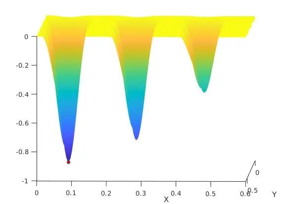
Unbounded case

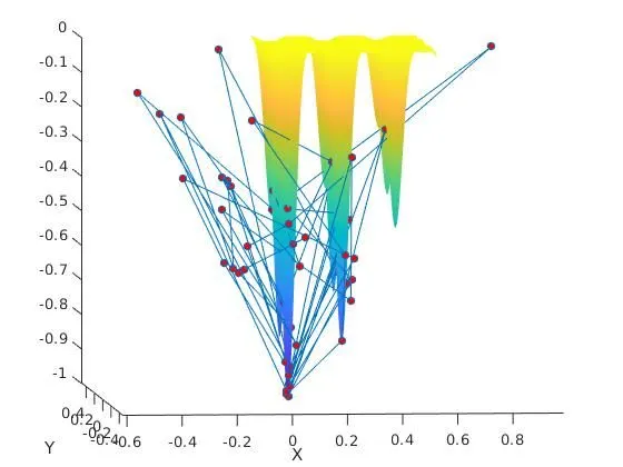
Bounded case

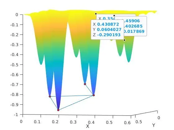
Bounded with limits