Week 4 - Genetic Algorithm

GENETIC ALGORITHM

AIM:

To write a code in MATLAB to optimise the stalagmite function using another optimisation algorithm:GA-Genetic Algorithm(in this case) and find the global maxima of the function.

CONCEPT:

• An Objective function is selected such that it exactly represents all the processes,calculations and variables associated. The objective function if solved gives a lot of solutions, but in order to find the optimal point for improved solution (with lesser resource wastage along with other paramaters that improve the desirability of the solution) an optimisation algorithm is required and it can be any proven algorithm. Here GA is used as an optimisation algorithm to optimise the Stalagmite function by taking it as the objective function-input.
• Note:GA always returns the minima of the objective function.So in order to obtain maxima suitable change is made to the objective function like changing the sign denotion.
• GA uses a search-based optimisation method that is governed by principles of genetics and natural selection.In MATLAB GA can solve constrained and unconstrained optimisation problems. It involves 3 basic steps and it starts after population initialisation.

1)Selection- In this process different highly fit parents are selected from the population. It can be compared to Roulette wheel selection where the probability of getting selected is directly proportional to the fitness; So selection of fitter individuals is predominant.

2)Cross-over- It is the process in which the solutions of the parents are crossed and given as solution for the offspring. There are many ways to do this one of it is one-point cross over method.

3)Mutation: This process avoids convergence between 2 solutions even if they are from the same parent and are most likely to be similar and there are several methods of mutations one of it is swap mutation where the chromosomes are swapped and the local minima is avoided due to convergence.

Syntax for ga:

[inputs,fval]=ga(@function,nvar,A,b,Aeq,beq,lb,ub,nonlcon,options)

1. inputs- this stores the input values given to the function for GA to optimise,x&y coordinates in this case.
2. fval- this stores the value of optimised solution from the objective function.
3. ga- it is the function name for calling the inbuilt ga solver.
4. function- it is the objective function that needs to be optimised.
5. nvar- it denotes the number of variables in the function.
6. A,b- this helps the GA to also find local minima 'x' to the function, subject to linear inequalities A*x ≤ b
7. Aeq,beq- this also helps GA to fing=d local minima 'x' to the function subject to linear inequalities Aeq*x = beq and A*x ≤ b
8. lb,ub- this sets the boundaries for the GA solver to operate and give solutions within the range lb ≤ x ≤ ub.
9. nonlcon- it imposes constraints on the minimisation if set. This deals with nonlinear inequalities and equalities.
10. options- this helps in changing the default optimisation parameters and setting customised values according to the needs of user.E.g: Editing the default population size from 50 to any natural number within the sample space this is coded seperately using optimoption function.

Termination Condition For GA:

The GA run end is determined by the termination condition. Intially GA progresses very fast but after few iterations the changes in value become very small. The termination condition should be in such a way that is renders a solution close to Optimal value.

Usually one of the following is used as termination condition:

1. No improvement in solution for n- generations.
2. When the absolute number of Generations are reached.
3. When the objective funvtion reaches a certain predefined value.

STALAGMITE FUNCTION: The Stalagmite function is a formulated mathematical model that takes 2 inputs namely x&y. Thus it is easily used for demonstrating our search space based optimisation algorithm.The Stalagmite function is given by the following formulae:

As already mentioned the Stalagmite formula has to be modified for GA to return maxima so the sign denotion of the final function is changed.Thus, f(x,y)= - f1x*f2x*f1y*f2y

This inverts the orientation of the total output plot. Thus the minima in the sign denotion changed plot is found out by GA and after that the sign is reversed and thus it becomes maxima.

STALAGMITE CODE BLOCK:

%Stalagmite Code:
function [F]=Stalagmite(input_vector)
x=input_vector(1);
y=input_vector(2);
f1x=(sin((5.1*pi*x)+0.5))^6;
f1y=(sin((5.1*pi*y)+0.5))^6;
f2x=exp((-4*log(2))/0.64*(x-0.0667)^2);
f2y=exp((-4*log(2))/0.64*(y-0.0667)^2);
[F]=-f1x*f1y*f2x*f2y;
end

MAIN PROGRAM:

clear all
close all
clc
%Defining search space:
x=linspace(0,0.6,150);
y=linspace(0,0.6,150);
%Creating 2D mesh:
[xx,yy]=meshgrid(x,y);

%Running Stalagmite-(Objective Function) within the search space: 
for i=1:length(xx)
    for j=1:length(yy)
        input_vector(1)=xx(i,j);
        input_vector(2)=yy(i,j);
        f_stalagmite(i,j)=Stalagmite(input_vector);
    end 
end

%Genetic Algorithm  Optimisation:
Iterations=50;

%Study 1-Basic and Unbounded Inputs:
tic;
for i=1:Iterations
    [input_1(i,:),f_ga_1(i,:)]=ga(@Stalagmite,2);
    x_ga_1(i)=input_1(i,1);
    y_ga_1(i)=input_1(i,2);
end
%Plotting:
figure(1)
subplot(2,1,1)
surfc(xx,yy,-f_stalagmite) %Sign denotion is reversed to obtain correct plot
shading interp %To remove shading
hold on
xlabel('xvalues')
ylabel('yvalues')
zlabel('Function Value')
plot3(x_ga_1,y_ga_1,-(f_ga_1),'marker','o','markersize',3,'markerfacecolor','r') %To plot all the stalagmite values generated on surface
title('Study-1')
subplot(2,1,2)
plot(-f_ga_1)
xlabel('Iterations')
ylabel('GA Function Values')
%To Display Global Maxima And it's Coordinates:
fopt_1=max(-(f_ga_1)); %Global Maxima for study 1
[row,col]=find(f_ga_1==-fopt_1);%Address/Index of max value(fopt_1) in the f_ga_1 array
opt_x_coordinate_1=input_1(row,1); %Value of X coordinate of search space from f_ga_1 array
opt_y_coordinate_1=input_1(row,2); %Value of Y coordinate of search space from f_ga_1 array
Study1_Time=toc;
Result_STUDY1=['Global Maxima for Study 1 = ',num2str(fopt_1),' At x =' ,num2str(opt_x_coordinate_1),' & y =',num2str(opt_y_coordinate_1),'  Time Elapsed =',num2str(Study1_Time)];


%Study 2-Bounded Inputs:
tic;
for i=1:Iterations
    [input_2(i,:),f_ga_2(i,:)]=ga(@Stalagmite,2,[],[],[],[],[0,0],[0.6,0.6]);
    x_ga_2(i)=input_2(i,1);
    y_ga_2(i)=input_2(i,2);
end
%Plotting:
figure(2)
subplot(2,1,1)
surfc(xx,yy,-f_stalagmite)
shading interp %To remove shading
hold on
xlabel('xvalues')
ylabel('yvalues')
zlabel('Function Value')
plot3(x_ga_2,y_ga_2,-(f_ga_2),'marker','o','markersize',3,'markerfacecolor','r') %To plot all the stalagmite values generated on surface
title('Study-2')
subplot(2,1,2)
plot(-f_ga_2)
axis([0 50 0 1.5])
xlabel('Iterations')
ylabel('GA Function Values')
%To Display Global Maxima And it's Coordinates:
fopt_2=max(-(f_ga_2)); %Global Maxima for study 1
[row,col]=find(f_ga_2==-fopt_2);%Address/Index of max value(fopt_1) in the f_ga_1 array
opt_x_coordinate_2=input_2(row,1); %Value of X coordinate of search space from f_ga_1 array
opt_y_coordinate_2=input_2(row,2); %Value of Y coordinate of search space from f_ga_1 array
Study2_Time=toc;
Result_STUDY2=['Global Maxima for Study 2 = ',num2str(fopt_2),' At x =' ,num2str(opt_x_coordinate_2),' & y =',num2str(opt_y_coordinate_2),'  Time Elapsed =',num2str(Study2_Time)];


%Study 3-Increasing Population size from (default) 50->170:
tic;
options=optimoptions('ga','PopulationSize',170);
for i=1:Iterations
    [input_3(i,:),f_ga_3(i,:)]=ga(@Stalagmite,2,[],[],[],[],[0,0],[0.6,0.6],[],options);
    x_ga_3(i)=input_3(i,1);
    y_ga_3(i)=input_3(i,2);
end
%Plotting:
figure(3)
subplot(2,1,1)
surfc(xx,yy,-f_stalagmite)
shading interp %To remove shading
hold on
xlabel('xvalues')
ylabel('yvalues')
zlabel('Function Value')
plot3(x_ga_3,y_ga_3,-(f_ga_3),'marker','o','markersize',3,'markerfacecolor','r') %To plot all the stalagmite values generated on surface
title('Study-3')
subplot(2,1,2)
plot(-f_ga_3)
axis([0 50 0 1.5])
xlabel('Iterations')
ylabel('GA Function Values')
%To Display Global Maxima And it's Coordinates:
fopt_3=max(-(f_ga_3)); %Global Maxima for study 1
[row,col]=find(f_ga_3==-fopt_3);%Address/Index of max value(fopt_1) in the f_ga_1 array
opt_x_coordinate_3=input_3(row,1); %Value of X coordinate of search space from f_ga_1 array
opt_y_coordinate_3=input_3(row,2); %Value of Y coordinate of search space from f_ga_1 array
Study3_Time=toc;
Result_STUDY3=['Global Maxima for Study 3 = ',num2str(fopt_3),' At x =' ,num2str(opt_x_coordinate_3),' & y =',num2str(opt_y_coordinate_3),'  Time Elapsed =',num2str(Study3_Time)];

%To display results in Command Window:
fprintf('nn');
disp(Result_STUDY1)
disp(Result_STUDY2)
disp(Result_STUDY3)

CODE EXPLANATION:

Appropriate comment lines are added for better understanding;

3 different studies are considered with different improvised constraints so that the GA gives the best optimum solution for almost all the iterations.

1. Basic and Unbounded Inputs
2. Bounded Inputs
3. Bounded Inputs with Increased polpulation size

The GA code is made to run and terminate 50 times and the values of all the iterations are stored and the overall best value is then returned as optimised solution for maxima.

Appropriate sign conventions and proper are carefully used to exactly denote and represent correct values.

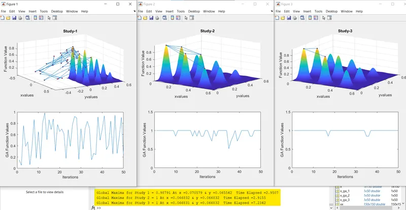
The result returns Global maxima for all three studies along with the coordinates they occur (in the search space - model generated by Stalagmite) and the time taken for optimisation in the command window.

OUTPUT:

STUDY1: Unbounded Inputs:

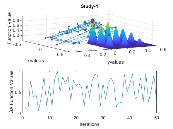
It can be seen that the optimisation doesn't have any bounds or limits to its search space thus majority of points optimised are outside study zone and large deviations from ideal solution is observed. Thus a boundary constraint was necessary.

STUDY2: Bounded Inputs:

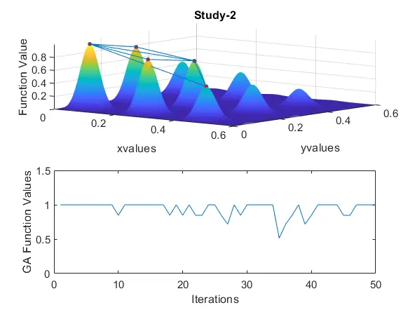
Still it can be observed that there are considerable amount of deviations from optimum value for different iterations,so it can be further improved by adding more population size rather than the default 50 population size.

STUDY3: Bounded Inputs with Increased polpulation size:

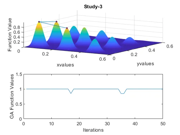
Now it can be seen that the solution is highly optimised with only negligible deviations from optimum value thus Global Maxima is more predominent than in other graphs where local minimas and maximas prevail.But this is the most time consuming of all studies but the accuracy of solution is good for almost all iterations.

Command Window Output:

All plots and Output for Visual Comparison of Different studies and their effectiveness in optimisation:

ERRORS AND CORRECTIONS:

1)Plotting error:

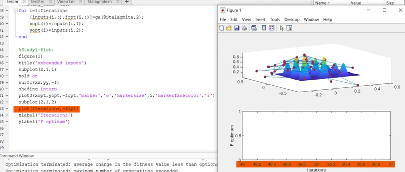
If the x axis is being specified it interrupts with the subplot command and proper values are not displayed.

Correction:Only the y axis is specified. The plot appears correctly as shown in output.

2)Array assigning error:

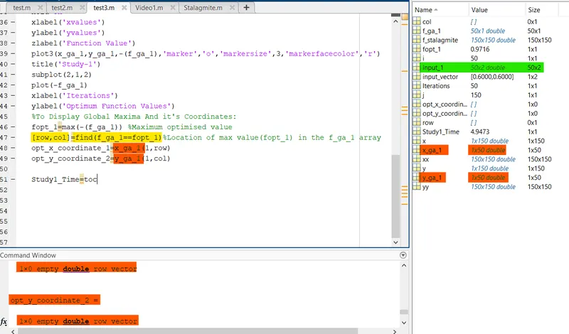
Instead of assigning coordinates to the variables in lines 48,49 from the base source array of find command the 'input_1' x_ga_1 andy_ga_1 were assigned since it had the x and y coordinates directly, and it resulted in creation of empty vectors that are useless.

Correction: The actual base array input_1 is used and the program is run to give proper output.

3)Indexing Errors:

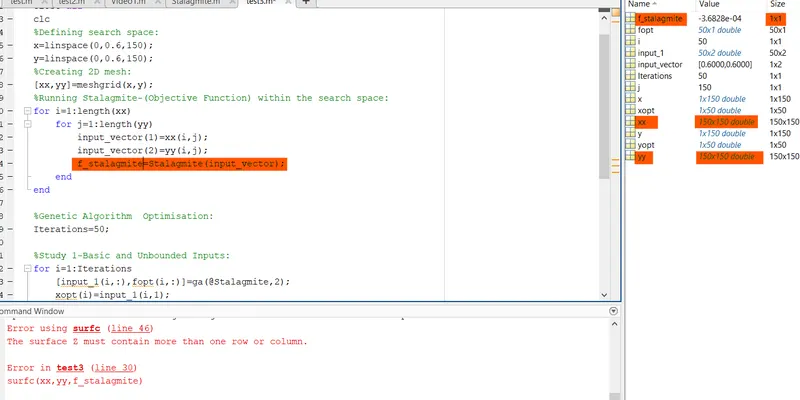
The f_stalagmite was not properly indexed causing the Stalagmite generation model impossible, since it started overwriting the value each time.

Correction:Properly indexed the variable is coded in program for proper model by preventing overwriting.

CONCLUSION:

The Stalagmite model was generated for a given search space and was taken as objective function and optimised using Genetic Algorithm as optimising algorithm under 3 different cases of study. The Global maxima was found and the related graphs were plotted. The Genetic Algorithm and its syntax was elaborated after studying and solid understanding of concepts.The code is proven to deliver the same result for multiple executions.