Week 4 - Genetic Algorithm

GENETIC ALGORITHM AND OPTIMIZATION USING MATLAB

OBJECTIVE:

• To understand the concept of a genetic algorithm.
• To find out information regarding stalagmite function and ways to optimize it.
• Write a code to optimize the stalagmite function and find the global maxima of the function.
• To explain the concept of a genetic algorithm.
• To make sure the code gives the same output, even if it is made to run several times.
• To plot graphs for all 3 studies and for F maximum vs no. of iterations.

INTRODUCTION

A genetic algorithm (GA) is an optimization technique used to solve nonlinear or non-differentiable optimization problems. They use concepts from evolutionary biology to search for a global minimum- to an optimization problem. The name genetic algorithm comes from the fact that they are mimicking evolutionary biology techniques.

PROCEDURE:

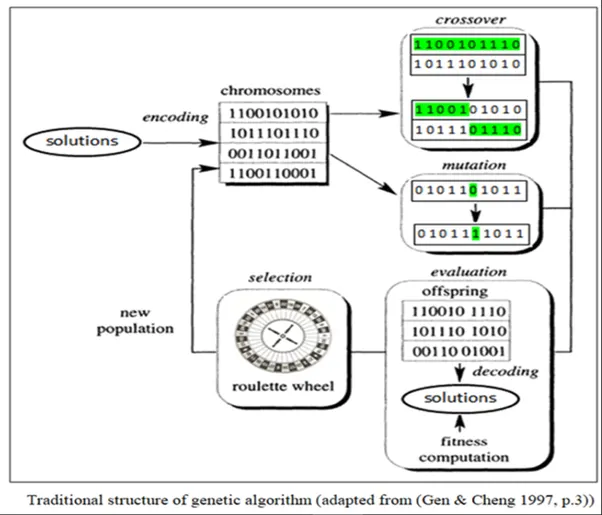
• Start with an initial generation of candidate solutions that are tested against the objective function.
• Subsequent generations evolve from the first generation through selection, crossover, and mutation.
• Selection --> It retains the best performing bit strings from one generation to the next generation. For example, if we have parent 1 and parent 2 performed well in the previous generation, they will continue to perform well in the next generation through the selection process.

Parent1 = [ 1 0 1 0 0 1 1 0 0 0 ]

Parent2 = [ 1 0 0 1 0 0 1 0 1 0 ]

• Crossover --> In this process we will create a child generation using similarities of both parent1 and parent2 generations.

Parent1 = [ 1 0 1 0 0 1 1 0 0 0 ]

Parent2 = [ 1 0 0 1 0 0 1 0 1 0 ]

Child = [ 1 0 0 0 0 1 1 0 1 0 ]

• MutationàIn this process we will use one parent and mutate certain variables to take on random values and create a child based on the mutation. Mutation allows genetic algorithms to kind of avoid falling into local minima and it relay helps them to explore the solution space well.

Parent1 = [ 1 0 1 0 0 1 1 0 0 0]

Child = [ 0 1 0 1 0 1 0 0 0 1]

Roulette Wheel Selection

• Roulette Wheel Selection In a roulette wheel selection, the circular wheel is divided as described before. before. A fixed point is chosen on the wheel circumference as shown and the wheel is rotated. rotated. The region of the wheel which comes in front of the fixed point is chosen as the parent. parent. For the second parent, parent, the same process is repeated.
• A fitter individual has a greater pie on the wheel and therefore a greater chance of landing in front of the fixed point when the wheel is rotated. rotated. Therefore, Therefore, the probability of choosing an individual depends directly on its fitness. Implementation wise, we use the following steps –

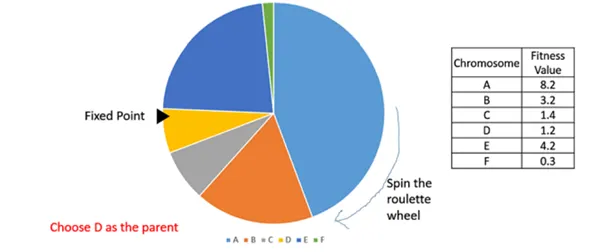
• Calculate S = the sum of a fitnesses.
• Generate a random number between 0 and S.
• Starting from the top of the population, population, keep adding the finesses to the partial sum P, till P
• The individual for which P exceeds S is the chosen individual.

Advantages of GA’s:

GA’s have various advantages that have made them immensely popular. These include –

• Does not require any derivative information (which may not be available for many real-world problems).
• Is faster and more efficient as compared to the traditional methods
• Has very good parallel capabilities.
• Optimizes both continuous and discrete functions and multi-objective problems
• Provides a list of “good” solutions and not just a single solution.
• Always gets an answer to the problem, which gets better over time.
• Always gets an answer to the problem, which gets better over time.

Limitations of GA’s:

Like any technique, GA’s also suffer from a few limitations. These include –

• GA’s are not suited for all problems, especially problems that are simple and for which derivative information is available.
• The fitness value is calculated repeated repeatedly which might be computationally expensive for some problems.
• Being stochastic, there are no guarantees on the optimality or the quality of the solution
• If not implemented properly, the GA may not converge to the optimal solution.

Equations Used in stalagmite function:

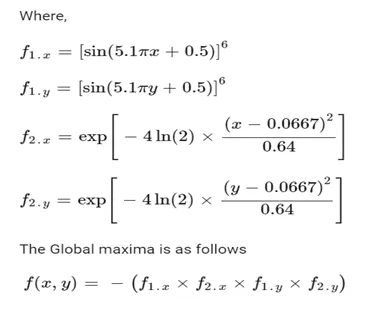
The Function is for the Genetic Algorithm of the global minima but in order to attain the maxima value the ‘-’ is placed before the equation.

F (x, y) = f1.x × f2.x ×f1.y × f2.y

Stalagmite function:

function input = stalagmite(X)
x = X(1);
y = X(2);
f1x = [sin(5.1*pi*x+0.5)].^6;
f2y = [sin(5.1*pi*y+0.5)].^6;
f3x = exp(-4*log(2)*((x-0.0667).^2/0.64));
f4y = exp(-4*log(2)*((x-0.0667).^2/0.64));
f = (f1x*f3x*f2y*f4y);
input = -f;

%'-ve' sign is used as the genetic algorithm 
% returns the global minima but we need the global maxima

end

MAINCODE:

clear all,
close all,
clc

x= linspace(0,1,200);
y=linspace(0,1,200);
num_case = 50;

[xx yy] = meshgrid(x,y);

%evaluating values of stalagmite function

for i = 1:length(xx)
    for j = 1:length(yy)
        input_vector(1) = xx(i,j);
        input_vector(2) = yy(i,j);
        f(i,j) = stalagmite(input_vector);
    end
end


% case study1, unbounded inputs
tic
for i = 1:num_case
    [inputs,f_opt(i)] = ga(@stalagmite,2);
    x_opt(i) = inputs(1); 
    y_opt(i) = inputs(2); 
end

study1 = toc
figure(1)
subplot(2,1,1)
hold on 
surfc (xx,yy,f)
shading interp
plot3(x_opt,y_opt,f_opt,'marker','o','markersize',5,'markerfacecolor','g');
title ('unbounded inputs')
xlabel(' x axis ')
ylabel (' y axis ')
zlabel(' function values ')

subplot(2,1,2)
plot(f_opt)
xlabel('x axis - iterations')
ylabel('y axis - min value')

% case study 2 using both upper and lower bounds
tic  
for i = 1:num_case
    [inputs,f_opt2(i)] = ga(@stalagmite,2,[],[],[],[],[0;0],[1;1]);
    x_opt2(i) = inputs(1); 
    y_opt2(i) = inputs(2); 
end


study2 = toc
figure(2)
subplot(2,1,1)
hold on 
surfc (xx,yy,f)
shading interp
plot3(x_opt2,y_opt2,f_opt2,'marker','o','markersize',5,'markerfacecolor','r');
title ('bounded inputs')
xlabel(' x axis ')
ylabel (' y axis ')
zlabel(' function values ')

subplot(2,1,2)
plot(f_opt2)
xlabel('x axis - iterations')
ylabel('y axis - min value')


% case study 3 increasing the population size with upper bound and lower
% bound
tic  
options = optimoptions('ga')
options = optimoptions(options,'populationsize',500)
for i = 1:num_case
    [inputs,f_opt3(i)] = ga(@stalagmite,2,[],[],[],[],[0;0],[1;1],[],[],options);
    x_opt3(i) = inputs(1);
    y_opt3(i) = inputs(2);
end

study3 = toc
figure(3)
subplot(2,1,1)
hold on 
surfc (xx,yy,-f)
shading interp
plot3(x_opt3,y_opt3,f_opt3,'marker','o','markersize',5,'markerfacecolor','k');
title ('bounded inputs with higher population size')
xlabel(' x axis ')
ylabel (' y axis ')
zlabel(' function values ')

subplot(2,1,2)
plot(f_opt3)
xlabel('x axis - iterations')
ylabel('y axis - max value')

Code Explanation:

• here we are creating values for x and y using the linspace command, we are creating 150 values between 0 to 0.8.
• we are using the mesh grid command cause meshgrid creates x and y values for 3D plots.
• we are using 50 iterations using 2 for loops and input arrays for x and y are created using stalagmite function.
• Time taken for the iteration is calculated using tic and toc commands.
• the ga inbuilt function does the genetic algorithm i.e. operations like selection, crossover, mutation, evaluation and roulette wheel. This creates new population for the defined stalagmite function for different iterations.
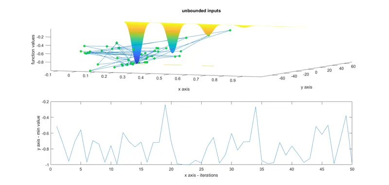
• now we are plotting the graph from the values we got from iterations of ga function, here we are making use of the subplot to plot 2 graphs in the same plot in which one is 3D plot for unbounded inputs and the other is 2D plot of optimum function.
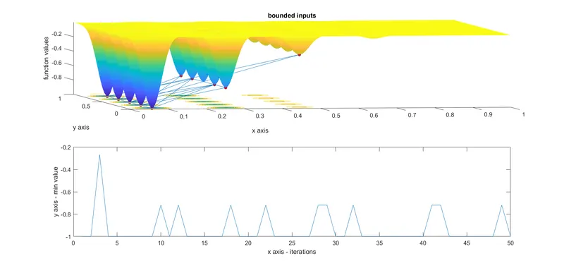
• Here it is difficult to obtain the global maxima as there are many points where the graph predicts the maxima. But here, we can obtain the local maxima of the function (for figure 1).

• Now, (for figure 2) we are running the iteration with upper and lower bound values.
• here f_opt is the function which stores optimum function values.
• x_opt2 and y_opt2 are the inputs values of the stalagmite for the case study 2.
• Similarly, ga inbuilt function does the genetic algorithm and the required graphs are plotted.

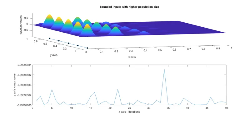
• For 3rd case study(for figure 3), we are increasing the population size to 500, now the iteration would take more time but we would end up with fewer maxima where we can obtain the global maxima.
• Similarly, ga inbuilt function does the genetic algorithm and the required graphs are plotted we give a negative sign in the surfc(xx,yy,-f) command so the graph is mirrored and we can obtain the global maxima.

Optimization

Optimization is a decision-making process, it helps to find the best results under a set of prioritized criteria or constraints. It is a procedure which is executed iteratively by comparing various solutions to an optimum or a satisfactory solution is found.

These include maximizing factors such as productivity, strength, reliability, efficiency, utilization, etc

Example:

Let’s take, you are designing a simply supported beam to withstand the load of 1-tonne, in this case, you need to consider the following parameters: Length, breadth, width, a factor of safety, weight, and stress-induced. Here optimization helps to find the best value for length, breadth, and width of the beam in such a way that the factor of safety, material consumed and stress-induced are within the limit.

MATLAB OPTIMIZATION

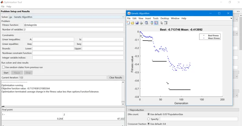
• we can use the optimization tool which is present in Matlab and use inbuilt GE to calculate our user-defined function
• here, I have optimized the @stalagmite function using an optimization tool in MatLab
• we can also input different variables, population size, upper bounds, lower bounds, fitness, etc.
• I have plotted fitness value vs generation. There are a whole lot of other graphs too which we can generate easily.

REFERENCES: 1. Genetic Algorithm explained!! : Skill Lync (freshdesk.com)

2. Genetic Algorithm - MATLAB & Simulink (mathworks.com)