Week 4 - Genetic Algorithm

Introduction:

Genetic Algorithm(GA):

The genetic algorithm is known as a search heuristic that is inspired by Charles Darwin's theory of natural evolution. This algorithm reflects the process of natural selection where the fittest individuals are selected for reproduction in order to produce offspring of the next generation. As shown in the flow chart, we need to choose an optimization algorithm process. GA is one of the optimization algorithm process. GA is commonly used to generate high-quality solutions to optimization and search problems by relying on biologically inspired operators such as mutation, crossover, and selection.

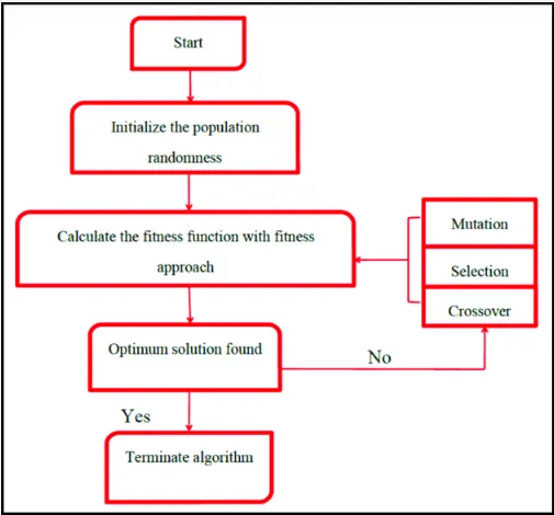
Selection: In this step, the parents are selected from the sample data points, the main objective of this process is select the highly fit individuals.

Cross over: It is the process of taking 2 parents solutions and producing the child from them. There are many ways to do cross over operations.

Mutation: This is carried out to maintain the genetic diversity from one generation of a population of chromosomes to the next. If the mutation is not performed, the chromosomes will become same to each other, then convergence take place soon and results in local minima.

General syntax for GA :-

b = Linear inequality constraints: real vector, if there are none, then [ ].

Aeq = Linear inequality constraints: real matrix, if there are none, then [ ].

beq = Linear inequality constraints: real matrix, if there are none, then [ ].

lb = lower bounds

ub = upper bounds

The function inputs are:

`f = f_(1x)* f_(1y) * f_(2x)*f_(2y)`

`f_(1x) = (sin(5.1pix+0.5))^6`

`f_(1y) = (sin(5.1piy+0.5))^6`

`f_(2x) = exp(-4ln(2)*(x-0.0667)^2/0.64)`

`f_(2y) = exp(-4ln(2)*(y-0.0667)^2/0.64)`

Function:

function [f] = stalagmite(input_vector);
   
   x = input_vector(1);
   y = input_vector(2);
   
   f1_x = (sin((5.1*pi*x)+0.5)).^6;
   f1_y = (sin((5.1*pi*y)+0.5)).^6;
   
   
   f2_x = exp(-4.*log(2)*(((x-0.0667).^2)/(0.64)));
   f2_y = exp(-4.*log(2)*(((y-0.0667).^2)/(0.64)));
   
   f = -(f1_x.*f2_x.*f1_y.*f2_y);
   
end

Code for unbounded and bounded inputs:

clear all
close all
clc

% Defining our search space
x = linspace(0,0.6,150);
y = linspace(0,0.6,150);

% creating a 2D mesh
[xx yy] = meshgrid(x,y);

% evaluating a stalagmite function
for i = 1:length(xx);
    for j = 1:length(yy);
        input_vector(1) = xx(i,j);
        input_vector(2) = yy(i,j);
        f(i,j) = stalagmite(input_vector);
    end    
end

 surfc(x,y,-f);
 xlabel('x values');
 ylabel('y values');
 shading interp

[inputs, fval] = ga(@stalagmite, 2)

tic        %% calculating the study time through tic and toc command
num_cases = 50;  %% GA runs for 50 iterations

% study 1 - statistical behavior
for i = 1:num_cases
    [inputs, fopt(i)] = ga(@stalagmite, 2);
    xopt(i) = inputs(1);
    yopt(i) = inputs(2);
end

study1_time = toc   %% displaying a time taken to evaluate

figure(1)
subplot(2,1,1)
hold on
surfc(x,y,f)
shading interp
xlabel('x axis')
ylabel('y axis')
plot3(xopt,yopt,fopt,'marker','o','markersize',5,'MarkerFaceColor','r')
title('unbounded inputs')
subplot(2,1,2)
hold on
plot(fopt)
xlabel('iterations')
ylabel('Function minimum')

tic
% study 2 - statistical behaviour - with upper and lower bounds
for i = 1:num_cases
    [inputs, fopt(i)] = ga(@stalagmite,2,[],[],[],[],[0;0],[1;1]);
    xopt(i) = inputs(1);
    yopt(i) = inputs(2);
end
study2_time = toc

figure(2)
subplot(2,1,1)
hold on
surfc(x,y,f)
shading interp
xlabel('x axis')
ylabel('y axis')
plot3(xopt,yopt,fopt,'marker','o','markersize',5,'MarkerFaceColor','r')
title('bounded inputs')
subplot(2,1,2)
plot(fopt)
xlabel('iterations')
ylabel('Function minimum')

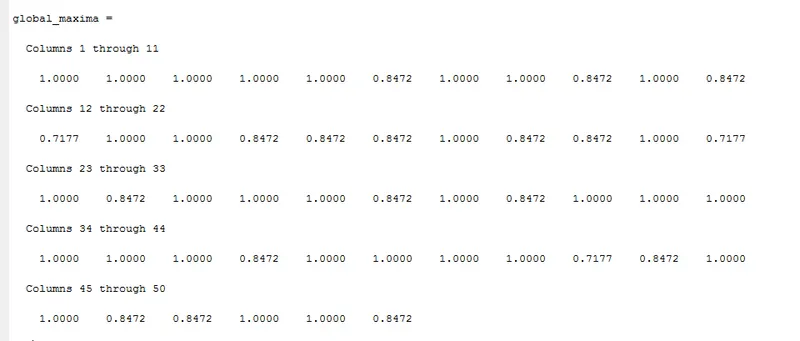
global_maxima = -fopt;

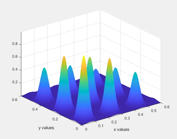
Study time1 = 6.4320

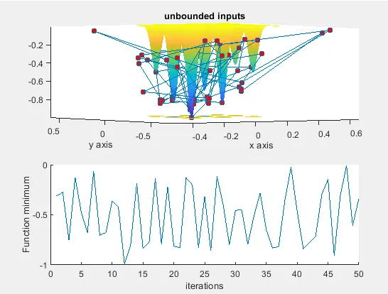
Study time2 = 14.9948

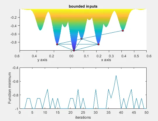
Global maxima:

Code for increase in the population size:

clear all
close all
clc

% Defining our search space
x = linspace(0,0.6,150);
y = linspace(0,0.6,150);

% creating a 2D mesh
[xx yy] = meshgrid(x,y);

% evaluating a stalagmite function
for i = 1:length(xx);
    for j = 1:length(yy);
        input_vector(1) = xx(i,j);
        input_vector(2) = yy(i,j);
        f(i,j) = stalagmite(input_vector);
    end    
end

 surfc(x,y,-f);
 xlabel('x values');
 ylabel('y values');
 shading interp

[inputs, fval] = ga(@stalagmite, 2)

tic        %% calculating the study time through tic and toc command
num_cases = 150;

% study 3 - increasing GA iterations
options = optimoptions('ga');
options = optimoptions(options,'populationsize',250);

tic
for i= 1 : num_cases
    [inputs, fopt(i)] = ga(@stalagmite,2,[],[],[],[],[0;0],[1;1],[],[],options);
    xopt(i) = inputs(1);
    yopt(i) = inputs(2);
end
study3_time = toc

figure(1)
subplot(2,1,1)
hold on
surfc(x,y,f)
shading interp
xlabel('x axis')
ylabel('y axis')
plot3(xopt,yopt,fopt,'marker','o','markersize',5,'MarkerFaceColor','r')
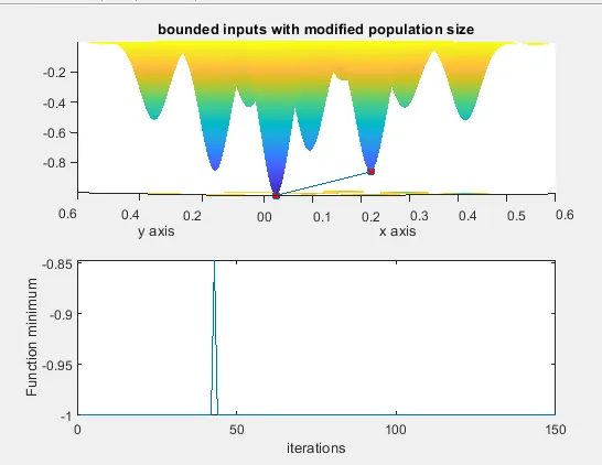
title('bounded inputs with modified population size')
subplot(2,1,2)
plot(fopt)
xlabel('iterations')
ylabel('Function minimum')

Study time3 = 170.38 for 150 iterations and population size is 250.

Conclusion:

From the above results the bounded samples with high population size are getting the accurate results. This is because the code shows the random values.

The global maxima is a function that can be found by inverting a function. The negative of the minimum values gives the global maxima.