Week 4 - Genetic Algorithm

Aim

The concept of genetic algorithm by referring to varius sources before you attend this challenge. Look out for information regarding stalagmite function and ways to optimise it.

Objectives of Project

• To write a code in MATLAB to optimise the stalagmite function and find the global maxima of the function.
• Clearly expalin the concept of genetic algorithm and also explain the syntax for ga in MATLAB in report.
• That code gives the same output, even if it is made to run several times.
• Plot graphs for all 3 studies and for F maximum vs no. of iterations.

Introduction of Genetic algorithm

1. Genetic Algorithm (GA) is a search-based optimization technique based on the principles of Genetics and Natural Selection. It is frequently used to find optimal or near-optimal solutions to difficult problems which otherwise would take a lifetime to solve. It is frequently used to solve optimization problems, in research, and in machine learning.

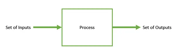
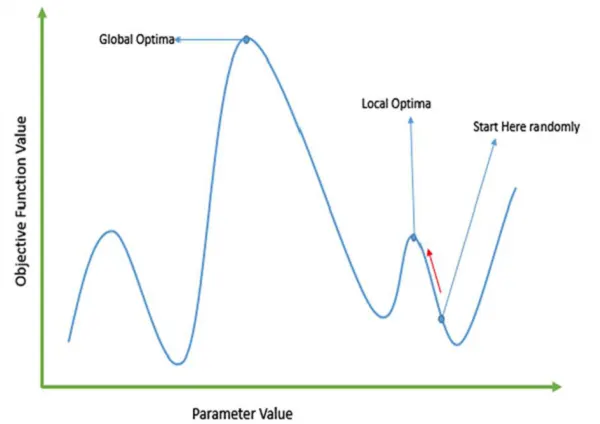
2. Nature has always been a great source of inspiration to all mankind. Genetic Algorithms (GAs) are search based algorithms based on the concepts of natural selection and genetics. GAs are a subset of a much larger branch of computation known as Evolutionary Computation.

3. Genetic Algorithms have the ability to deliver a “good-enough” solution “fast-enough”. This makes genetic algorithms attractive for use in solving optimization problems. The reasons why GAs are needed are as follows − There is a large set of problems, which are NP-Hard. What this essentially means is that, even the most powerful computing systems take a very long time (even years!) to solve that problem. In such a scenario, GAs prove to be an efficient tool to provide usable near-optimal solutions in a short amount of time.

Below shown the flow chart of genetic algorithm.

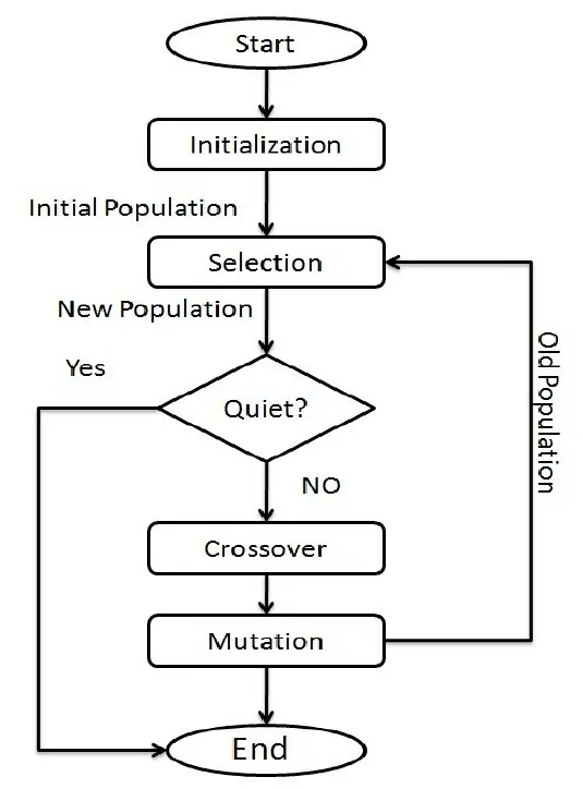
Phases in Genetic algorithm

Five phases are considered in a genetic algorithm.

1. Initial population
2. Fitness function
3. Selection
4. Crossover
5. Mutation

1. Initialization of Population(Coding)

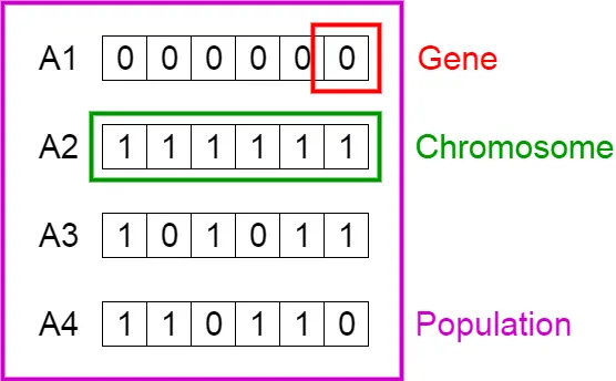
• Every gene represents a parameter (variables) in the solution. This collection of parameters that forms the solution is the chromosome. The population is a collection of chromosomes.
• Order of genes on the chromosome matters.
• Most of the time chromosomes are depicted in binary as 0’s and 1’s, but there are also other encodings possible.

2. Fitness Function

• Out of the available chromosomes, we have to select the best ones for the reproduction of offsprings, so each chromosome is given a fitness value.
• The fitness score helps to select the individuals which will be used for reproduction.

3. Selection

• The main goal of this phase is to find the region where the chances of getting the best solution are more.
• Inspiration for this is from the survival of the fittest.
• It should be a balance between exploration and exploitation of search space.
• GA tries to move the genotype to higher fitness in the search space.
• Too strong fitness selection bias can lead to sub-optimal solutions.
• Too little fitness bias selection results in unfocused search.
• Thus Fitness proportionate selection is used, which is also known as roulette wheel selection, is a genetic operator used in genetic algorithms for selecting potentially useful solutions for recombination.

4. Reproduction

Generation of offsprings happen in 2 ways:

• Crossover
• Mutation

a) Crossover

Crossover is the most vital stage in the genetic algorithm. During crossover, a random point is selected while mating a pair of parents to generate offsprings.

There are 3 major types of crossover.

• Single Point Crossover: A point on both parents’ chromosomes is picked randomly, and designated a ‘crossover point’. Bits to the right of that point are exchanged between the two parent chromosomes.
• Two-Point Crossover: Two crossover points are picked randomly from the parent chromosomes. The bits in between the two points are swapped between the parent organisms.
• Uniform Crossover: In a uniform crossover, typically, each bit is chosen from either parent with equal probability.

The new offspring are added to the population.

b) Mutation

In a few new offspring formed, some of their genes can be subjected to a mutationwith a low random probability. This indicates that some of the bits in the bit chromosome can be flipped. Mutation happens to take care of diversity among the population and stop premature convergence.

5. Convergence (when to stop)

Few rules which are followed which tell when to stop is as follows:

• When there is no improvement in the solution quality after completing a certain number of generations set before hand.
• When a hard and fast range of generations and time is reached.
• Till an acceptable solution is obtained.

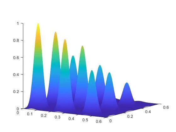
Stalagamite formula

The formula will be

`f(x,y) = f1x, f2x , f1y, f2y`

There will be

`f1x = [sin (5.1 pi x + 0.5)]^6`

`f1y = [sin (5.1 pi y + 0.5)]^6`

`f2x = exp[- 4 In(2) (x- 0.0667)^2/0.64]`

`f2y = exp[- 4 In(2) (y- 0.0667)^2/0.64]`

These above formula to calculate the stalagamite using function method.

Function method used genetic algorithm

function [f] = stalagamite(input_vector)
  
f1_x = (sin(5.1*pi*input_vector(1)+0.5))^6;
f1_y = (sin(5.1*pi*input_vector(2)+0.5))^6;
 
f2_x = exp(-4.*log(2)*(((input_vector(1)-0.0667).^2)/(0.64)));

f2_y = exp(-4.*log(2)*(((input_vector(2)-0.0667).^2)/(0.64)));

f = (f1_x.*f1_y.*f2_x.*f2_y);

end

Basic code for genetic algorithm

clear all
close all
clc

% defining our search space
x = linspace (0,0.6,150);
y = linspace (0,0.6,150);

% creating 2D dimensional mesh

[xx yy] = meshgrid(x,y);

% Evaluating the stalagmite function

for i = 1: length(xx);
  for j = 1: length(yy);
    
    input_vector(1) = xx(i,j);
    input_vector(2) = yy(i,j);
    f(i,j) = stalagamite(input_vector);
  end
  
end

surface (xx,yy,f)

shading interp

[inputs, fval] = ga(@stalagamite,2)

The reults will be

Main code

Genetic alagorithm code created based on different stage of using the plot.

clear all
close all
clc

% defining our search space
x = linspace (0,0.6,150);
y = linspace (0,0.6,150);

num_case = 50;

% creating 2D dimensional mesh

[xx yy] = meshgrid(x,y);


% Evaluating the stalagmite function
tic
for i = 1: length(xx)
  for j = 1: length(yy)
    
    input_vector(1) = xx(i,j);
    input_vector(2) = yy(i,j);
    f(i,j) = get_stalagmite(input_vector);
    
  end
  
end
study_time = toc

surfc(xx,yy,-f)
shading interp
xlabel('x value')
ylabel('y value')
title('stalagmite function')

% Evaluate the staistical behaviour stage 1
tic
for i = 1:num_case;
    [inputs, fopt(i)] = ga(@stalagamite,2);
        xopt(i) = inputs(1);
        yopt(i) = inputs(2);
end

study1_time = toc

figure(1)
subplot(2,1,1);
hold on
surfc(x,y,-f);
shading interp
plot3(xopt,yopt,-fopt,'marker','o','markersize',5,'markerfacecolor','g');
title('unbounded inputs');
subplot(2,1,2);
plot(fopt)
xlabel('iteration');
ylabel('function minimum');

% stage 2

% Evaluate the staistical behaviour 0f upper and lower bound
tic
for i = 1:num_case;
    [inputs, fopt(i)] = ga(@stalagamite,2, [],[],[],[],[0;0],[0.6;0.6]);
        xopt(i) = inputs(1);
        yopt(i) = inputs(2);
end

study2_time = toc

figure(2)
subplot(2,1,1);
hold on
surfc(x,y,f);
shading interp
plot3(xopt,yopt,-fopt,'marker','o','markersize',5,'markerfacecolor','g');
title('unbounded inputs');
subplot(2,1,2);
plot(-fopt)
xlabel('iteration');
ylabel('function minimum');


% stage 3

% Evaluate the staistical behaviour of GA iterations

options = optimoptions('ga');
options = optimoptions(options,'populationsize',170);
tic
for i = 1:num_case;
    [inputs, fopt(i)] = ga(@stalagamite,2, [],[],[],[],[0;0],[1;1],[],[],options);
        xopt(i) = inputs(1);
        yopt(i) = inputs(2);
end

study3_time = toc

figure(3)
subplot(2,1,1);
hold on
surfc(x,y,f);
shading interp
plot3(xopt,yopt,-fopt,'marker','o','markersize',5,'markerfacecolor','g');
title('unbounded inputs');
subplot(2,1,2);
plot(-fopt)
xlabel('iteration');
ylabel('function minimum');


global_maxima = -fopt

Stage 1 code

Here below shown the stage 1 code for behaviour stage.

% Evaluate the staistical behaviour stage 1
tic
for i = 1:num_case;
    [inputs, fopt(i)] = ga(@stalagmite,2);
        xopt(i) = inputs(1);
        yopt(i) = inputs(2);
end

study1_time = toc

figure(1)
subplot(2,1,1);
hold on
surfc(x,y,-f);
shading interp
plot3(xopt,yopt,-fopt,'marker','o','markersize',5,'markerfacecolor','g');
title('unbounded inputs');
subplot(2,1,2);
plot(fopt)
xlabel('iteration');
ylabel('function minimum');

Stage 2 code

Here we found the stage 2 for upper and lower bound. becasue here we didnt find better accuracy in stage 1.

% Evaluate the staistical behaviour 0f upper and lower bound
tic
for i = 1:num_case;
    [inputs2, fopt2(i)] = ga(@stalagmite,2, [],[],[],[],[0;0],[1;1]);
        xopt(i) = inputs2(1);
        yopt(i) = inputs2(2);
end

study2_time = toc

figure(2)
subplot(2,1,1);
hold on
surfc(x,y,f);
shading interp
plot3(xopt,yopt,-fopt2,'marker','o','markersize',5,'markerfacecolor','g');
title('unbounded inputs');
subplot(2,1,2);
plot(-fopt2)
xlabel('iteration');
ylabel('function minimum');

Stage 3 code

Here stage 3 code working for more accuracy for GA value to get better GA value. So we setup the population size 170. so we get accurate value of code.

% Evaluate the staistical behaviour of GA iterations

options = optimoptions('ga');
options = optimoptions(options,'populationsize',170);
tic
for i = 1:num_case;
    [inputs3, fopt3(i)] = ga(@stalagmite,2, [],[],[],[],[0;0],[1;1],[],[],options);
        xopt(i) = inputs3(1);
        yopt(i) = inputs3(2);
end

study3_time = toc

figure(3)
subplot(2,1,1);
hold on
surfc(x,y,f);
shading interp
plot3(xopt,yopt,-fopt3,'marker','o','markersize',5,'markerfacecolor','g');
title('unbounded inputs');
subplot(2,1,2);
plot(-fopt3)
xlabel('iteration');
ylabel('function minimum');


global_maxima = -fopt

Conclusion

Here Genetic algorithm based we get for population each year or some year once to find easily. This also used for various segments like automobile or survey etc.

genetic algorithm basicaly used to find out for global minimum used to find out by using (-) sign we find the global maxima from GA.