Week 3 - Solving second order ODEs

Aim

The ODE behaviour of the simple pandulum system code using MATLAB.

1) The way pendulum oscillates on newton 2nd law of motion.

2) ODE based on used for differential equation. To use ODE equation describes the ball position and oscillates in simple pendulum.

3) ODE is the key phenomena to solve the below given differential equation.

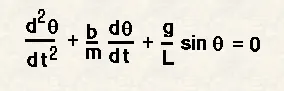
Based on equation we consider,

g = gravity in m/s2,

L = length of the pendulum in m,

m = mass of the ball in kg,

b=damping coefficient.

Introduction

A pendulum is a device that is found in wall clocks. It consists of a weight (bob) suspended from a pivot by a string or a very light rod so that it can swing freely. When displaced to an initial angle and released, the pendulum will swing back and forth with a periodic motion. By applying Newton’s second law of motion for rotational systems, the equation of motion for the pendulum may be obtained.

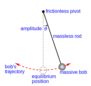
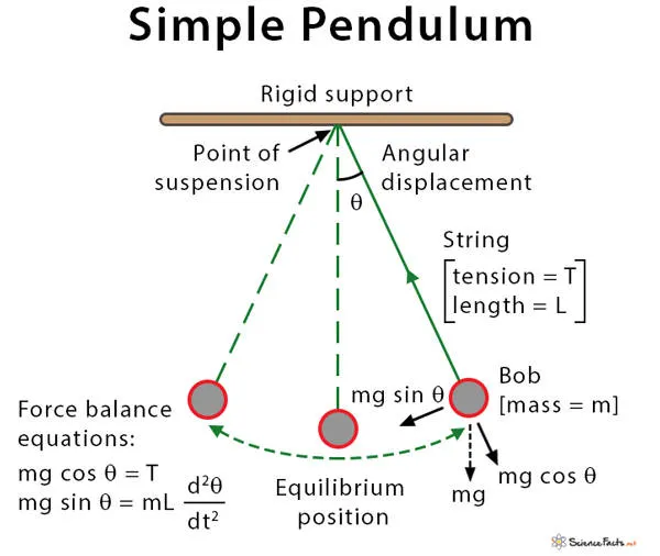
1) In above pendulum fig shows, the point of suspension is fixed. In below that string is fixed with bob or weight (mass m). From the certain length (l) used to oscillate the pendulum from one place to another place is called equilibirum position with taken time (t) of sec.

2) Provide some damping force from original position oscillates weight in the angle of θ. In the angle will vary for the "n" number of time. A simple pendulum has a heavy point mass (known as bob) suspended from a rigid support by a massless and inextensible string. When the bob from its mean position is pulled to one side and then released, the pendulum is set to motion and the bob moves alternately on either side of its mean position.

3) In the fig shows time period of pendulum doesn't depend on the size or mass of the pendulum, it depends on the length of the pendulum and factor of earth's gravity. The fig shows the tagential and radial components of the gravitational force in pendulum. The radial component is exactly balanced by the force exerted by the string, so only relevant force producing in the tangential component of gravitational force. So we can neglect the daming force.

ODE Equation for simple pendulum

1) ODE is the differential equation contains one or more functions of one independent vaiables and derivatives those function.

Here,

θ = θ1

`therefore``(d theta) / dt` = `(d theta1) / dt` = `theta2` `----------> (1)`

`(d^2 theta) / dt^2` = `(d^2 theta1) / dt^2` = `d/dt((d theta1) / dt)` = `d/dt(theta2)` `--------------->(2)`

Next step equation 1 & 2 Implementing in the below equation

`(d^2 theta) / dt^2 + b/m d_theta/dt + g/l sintheta = 0`

Now, θ = θ1

`(d^2 theta) / dt^2 + b/m d_(theta1)/dt + g/l sintheta1 = 0`

We have from equation (2)

`(d^2 theta) / dt^2 = d_(theta2)/dt`

So,

`d_(theta2)/dt + b/m d_(theta1)/dt + g/l sintheta1 = 0`

`d_(theta2)/dt = -b/m d_(theta1)/dt - g/l sintheta1`

We have equation (1) `(d theta1) / dt = theta2`

So,

`d_(theta2)/dt = -b/m theta2 - g/l sintheta1`

we have `d/dt[theta1;theta2]` is the solution vector

So,

`d/dt[theta1;theta2] = [theta2; -b/m theta2 - g/l sintheta1]`

For these we need to write the basic function program code in MATALB

function [dtheta_dt] = ode_func(t,theta,b,g,l,m)

theta1 = theta(1)
theta2 = theta(2)
dtheta1_dt = theta2;
dtheta2_dt = -(b/m)*theta2 - (g/l)*sin(theta1);
dtheta_dt = [ dtheta1_dt; dtheta2_dt];


end

These above program to calculate the solution vector.

Main code Oscillation create code for MATLAB.

Here just a simple program without pendulum movement or any animation created code shown below.

clear all
close all
clc

% Inputs

% damping coefficient
b = 0.05;

% gravity (m/s^2)
g = 9.81;

% length of spring (m)
l = 1;

% mass of ball (kg)
m = 1;

% initial condion
% initail displacement of pendulum and initial velocity of pendulum

theta_0 = [0;3];

% time points
% pendulum spring oscillates o to 20 sec 

t_span = linspace(0,20,600);

% solve ODE function
% ode45 is the inbuit solving default in matlab

[t,results] = ode45(@(t,theta) ode_func(t,theta,b,g,l,m),t_span, theta_0);

plot(t,results(:,1));
hold on
plot(t,results(:,2));
xlabel('time (sec)');
ylabel('angular displacement & angular velocity')

grid on

Here ode45 is the inbuilt solving differential equation in MATLAB.

Below showing plot for Resonance of pendulum.

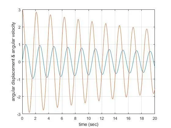
For animation of pendulum we are going to use "for loop" statement in code. Because time of oscillation in different period of time and different angle.

Code for "For loop" and animation

% for loop define the motion of pendulum
ct = 1
for i= 1: length (results(:,1));
    x_start = 0;
    y_start = 0;
    x_end = l*sin (results(i,1));
    y_end = -l*cos (results(i,1));
    
    %plot for animation
    figure(2)
        plot([x_start x_end],[y_start y_end], 'linewidth', 3, 'color', 'b');
        hold on
        plot([-1 1], [0 0], 'linewidth', 4, 'color', 'r');
        hold on
                        
        plot(x_end, y_end, 'marker','o', 'markersize',25,'markerfacecolor','g')
        title('Resonance of pendulum')
        axis([-1.5 1.5 -1.5 0]);
        pause(0.1)
        M(ct) = getframe(gcf);
        ct=ct+1;
        
        hold off
        
    
end

Here we are using "for loop" command due to define the motion of pendulum. Because we gave time span upto 600 times.

t_span = linspace(0,20,600);

Here x_start & y_start is 0. But while x_end & y_end based on angle is changed.

Final code

clear all
close all
clc

% Inputs

% damping coefficient
b = 0.05;

% gravity (m/s^2)
g = 9.81;

% length of spring (m)
l = 1;

% mass of ball (kg)
m = 1;

% initial condion
% initail displacement of pendulum and initial velocity of pendulum

theta_0 = [0;3];

% time points
% pendulum spring oscillates o to 20 sec 

t_span = linspace(0,20,600);

% solve ODE function
% ode45 is the inbuit solving default in matlab

[t,results] = ode45(@(t,theta) ode_func(t,theta,b,g,l,m),t_span, theta_0);

plot(t,results(:,1));
hold on
plot(t,results(:,2));
title('Resonance of pendulum')
legend('angular displacement', 'angular velocity')
xlabel('time (sec)');
ylabel('Y axis')

% for loop define the motion of pendulum
ct = 1
for i= 1: length (results(:,1));
    x_start = 0;
    y_start = 0;
    x_end = l*sin (results(i,1));
    y_end = -l*cos (results(i,1));
    
    %plot for animation
    figure(2)
        plot([x_start x_end],[y_start y_end], 'linewidth', 3, 'color', 'b');
        hold on
        plot([-1 1], [0 0], 'linewidth', 4, 'color', 'r');
        hold on
        
        
        
        plot(x_end, y_end, 'marker','o', 'markersize',25,'markerfacecolor','g')
        title('Resonance of pendulum')
        axis([-1.5 1.5 -1.5 0]);
        pause(0.1)
        M(ct) = getframe(gcf);
        ct=ct+1;
        
        hold off
        
    
end
grid on

% Animation for resonance of pendulum
movie(M)
videofile = VideoWriter('Resonance of pendulum.avi','uncompressed AVI');
open(videofile)
writeVideo(videofile,M)
close(videofile)

Result

Resonance of pendulum video file attached.

Error

#1

I face some of the problem for execute the resonance of pendulum hold command made it off. so each and every displacement it shows the pendulum holding some sec then it release. below pic shown exactly.

plot(x_end, y_end, 'marker','o', 'markersize',25,'markerfacecolor','g')
        title('Resonance of pendulum')
        axis([-1.5 1.5 -1.5 0]);
        pause(0.1)
        M(ct) = getframe(gcf);
        ct=ct+1;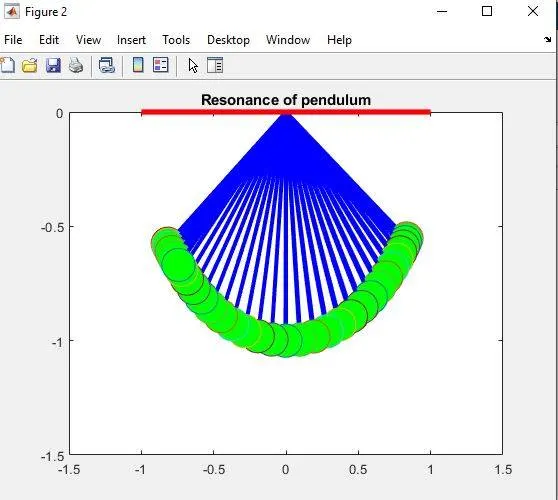

Conclusion

Here simple way the pendulum moves depends on the Newtons second law using MATLAB code using ODE equation to solve the problems and got final output. Similarly, there are hundreds of ODEs that describe key phenomena and to solve these equations.