Week 4 - Genetic Algorithm

AIM:

To write a MATLAB program to optimise the stalagmite function and find the global maxima of the function.

GOVERNING EQUATIONS:

1. `f(x,y) = f_1,xf_2,xf_1,yf_2,y`
2. `f_1.x = [sin(5.1pix+0.5)]^6`
3. `f_1.y = [sin(5.1piy+0.5)]^6`
4. `f_2,x = exp[-4ln(2)((x-0.6667)^2/0.64)]`
5. ``f_2,y = exp[-4ln(2)((y-0.6667)^2/0.64)]``

OBJECTIVE:

The objective of the project is to learn the concept of optimization of the stalagmite function using the genetic algorithm in MATLAB.

PROGRAMMING LANGUAGE USED:

MATLAB

CODE SAMPLE:

The Stalagmite function

function [A] = stalagmite(input_vector) %Defining the function

a = input_vector(1);
b = input_vector(2);

%Calculating the terms in the function

f1x = (sin((5.1*pi*a)+0.5)).^6;
f1y = (sin((5.1*pi*b)+0.5)).^6;

f2x = exp(-4*log(2)*((a-0.06667).^2/0.64));
f2y = exp(-4*log(2)*((b-0.06667).^2/0.64));

A = -(f1x.*f1y.*f2x.*f2y); %Negative sign used to calculate the global maxima

end

Optimizing stalagmite function using Genetic algorithm (GA)

clear all
close all
clc

%Defining the inputs
x = linspace(0,0.6,150);
y = linspace(0,0.6,150);

num_cases = 50;

%Creating 2x2 matrix of the input matrices
[xx,yy] = meshgrid(x,y);


for i = 1:length(xx)
    for j = 1:length(yy)

        input_vector(1) = xx(i,j);
        input_vector(2) = yy(i,j);
        A(i,j) = stalagmite(input_vector);

    end
end

%Study 1 - Unbounded inputs

tic

for i = 1:num_cases

    [inputs,fopt(i)] = ga(@stalagmite,2);
    xopt(i) = inputs(1);
    yopt(i) = inputs(2);

end

study1_time = toc %Caclculating time taken for execution of code

figure(1)
subplot(2,1,1)
hold on

surfc(x,y,-A)
shading interp

xlabel('X values')
ylabel('Y values')

plot3(xopt,yopt,-fopt,'marker','O','markersize',5,'markerfacecolor','r');

title('Unbounded inputs')
subplot(2,1,2)

plot(-fopt)

xlabel('Iterations')
ylabel('Function maximum')

%Study 2 - Bounded inputs

tic

for i = 1:num_cases

   [inputs,fopt(i)] = ga(@stalagmite,2,[],[],[],[],[0;0],[0.3;0.3]);
    xopt(i) = inputs(1);
    yopt(i) = inputs(2);

end

study2_time = toc %Caclculating time taken for execution of code

figure(2)
subplot(2,1,1)
hold on

surfc(x,y,-A)
shading interp

xlabel('X values')
ylabel('Y values')

plot3(xopt,yopt,-fopt,'marker','O','markersize',5,'markerfacecolor','r');

title('Bounded inputs')
subplot(2,1,2)

plot(-fopt)

xlabel('Iterations')
ylabel('Function maximum')

options = optimoptions(@ga);
options = optimoptions(@ga,'populationsize',200);

%Study 3 - Bounded inputs with population increased

tic

for i = 1:num_cases

   [inputs,fopt(i)] = ga(@stalagmite,2,[],[],[],[],[0;0],[0.3;0.3],[],[],options);
   xopt(i) = inputs(1);
   yopt(i) = inputs(2);

end

study_time3 = toc %Caclculating time taken for execution of code

figure(3)
subplot(2,1,1)
hold on

surfc(x,y,-A)
shading interp

xlabel('X values')
ylabel('Y values')

plot3(xopt,yopt,-fopt,'marker','O','markersize',5,'markerfacecolor','r');

title('Bounded inputs with increased population')
subplot(2,1,2)

plot(-fopt)

xlabel('Iterations')
ylabel('Function maximum')

ALGORITHM:

First, the inputs are given using the linspace command. They are then converted to a 2x2 matrix using the meshgrid command. Then we have the 2 FOR loops inside which we call the stalagmite function. The stalagmite function is defined in a separate file ‘stalagmite.m’. The purpose of having 2 for loops is to perform a particular task which includes 2 variables by keeping one variable constant and perform operation on the other variable. The value of the stalagmite function is calculated and stored in a variable which is later used to plot. Then the global maxima of the function is found by carrying out 3 studies by narrowing to the optimized solution.

Syntax of Genetic algorithm (GA):

The genetic algorithm function is an in-built function in MATLAB which has different types of syntax. The function is called by using ‘ga’. Some of the syntax are explained below:

• x = ga(fun,nvars)

This command returns the local minimum of the specified function. It takes the function ‘fun’ and the number of design variables ‘nvars‘ in the function.

• x = ga(fun,nvars,A,b)

This command returns the local minimum of the specified function subject to linear inequalities A*x< b

• x = ga(fun,nvars,A,b,Aeq,beq)

This command returns the local minimum of the specified function subject to the linear equalities Aeq*x = beq and A*x ≤ b. The values for A & b can be set as ‘[ ]’ if no linear equalities exist.

• x = ga(fun,nvars,A,b,Aeq,beq,lb,ub)

This command returns the local minimum of the specified function with a set of lower & upper bounds ‘lb’ & ’ub ‘on the design variables.

• x = ga(fun,nvars,A,b,[],[],lb,ub,nonlcon,IntCon,options)

This command returns the local minimum of the specified function by minimizing the default optimizing parameters replaced by values in ‘options’. The options can be created using the ‘optimoptions’ command.

• optimoptions(SolverName,Name,Value)

This command is used to give options to the ga. It takes the solver name, name of the option and its value as inputs.

EXPLANATION:

First, the inputs for defining the workspace are given. It is given using the linspace command. The values are stored in variables x and y. A 2-D matrix of the same is created using the meshgrid command. It is then stored in arrays xx and yy. Then the value for the stalagmite function is found by with the help of two for loops. The loop counter variables for the loops are i and j. They start from 1 and go up to the length of xx and yy respectively. Then the value of the stalagmite function is computed by calling the function. The formula for the stalagmite function is created in a separate MATLAB function ‘stalagmite’.

Next, we carry out the three studies. In the first study we have no bounds for the inputs. The population is set as 150. We find the global maximum by giving input as the function and number of design variables. The time taken for this computation is calculated by using the tic and toc commands. It is stored in the variable study1_time. Then, we create a figure window and create a surface plot in it. The local maxima are also plot in the surface plot. The surface plot is made in the figure window 1 as a subplot. In another subplot, we plot the function maximum versus No. of Iterations.

In the second study, we calculate the global maxima by giving upper and lower bounds along with the function and no. of design variables. The population is maintained as 150. As in the previous case, the time taken to compute is calculated with the help of tic and toc commands. The time is stored in the variable study2_time. Once the global maxima is calculated, we do the plots as in the previous study. For this study, we do the plots in a separate figure window.

Finally, in the third study we calculate the global maxima by giving the same upper & lower bounds but with an increased population. In this case, the population is set as 200. As in previous studies, the time for computation is calculated using tic and toc commands and stored in the variable study3_time. For this purpose, we use the optimoptions command. It enables us to change the default population of 150 and implements this population change in the ga. The plots are plot using the plot command as in the previous cases.

RESULTS:

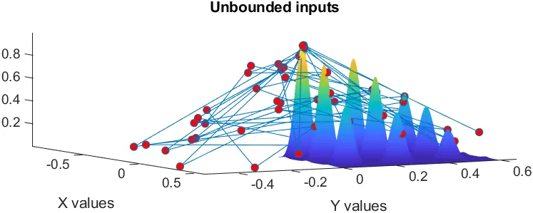
In the first surface plot, we can see that there are many points plot. These are the maxima. Since there are unbounded inputs the output we obtain is not accurate.

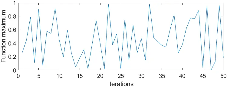
Also from the above 2-D plot, we can see that the function maximum (global maxima) is changing with the number of iterations.

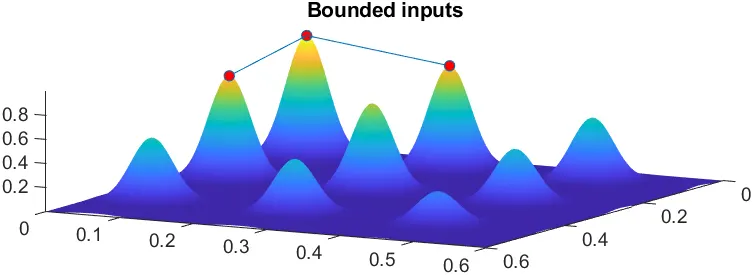
In the second surface plot, we can see that the no. of points on the peak is significantly reduced from the previous study. We have narrowed at the solution.

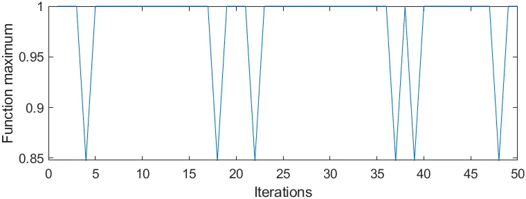
From the 2-D plot, we can see that the function maximum (global maxima) is changing less as compared to the previous study. It is quite constant.

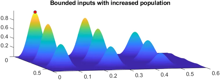
In the third surface plot, we can see that we have obtained the exact global maxima for the function. We only have one point marked, which is the global maxima.

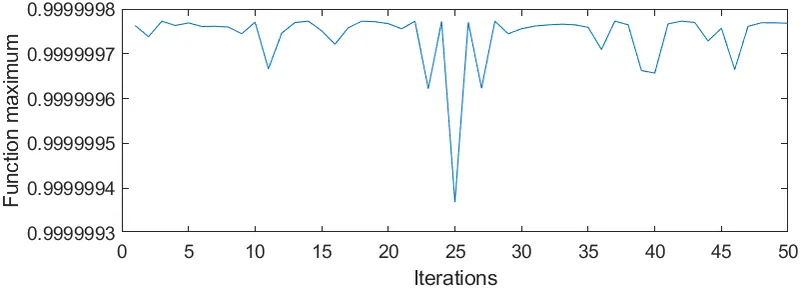
Even in the 2-D plot, the changes are very less. It indicates we have reached to an optimum point.

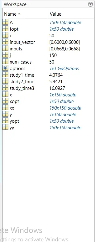
From the output obtained in the workspace, we can see that the time taken for each study to process is more than the previous one.

CONCLUSION:

Thus the genetic algorithm was used to solve the stalagmite function to optimize the function and find the global maxima. The output surface and 2-D plots obtained are shown. The time taken for each study is also recorded and obtained in the workspace. We can conclude that by increasing the number of iterations, population and setting lower and upper bounds, we obtain the result for global maxima accurately.