Week 4 - Genetic Algorithm

AIM

To write a code in MATLAB to optimise the stalagmite function and find the global maxima of the function.

GENETIC ALGORITHM

A genetic algorithm (GA) is a method for solving both constrained and unconstrained optimization problems based on a natural selection process that mimics biological evolution. The algorithm repeatedly modifies a population of individual solutions. At each step, the genetic algorithm randomly selects individuals from the current population and uses them as parents to produce the children for the next generation. Over successive generations, the population "evolves" toward an optimal solution.

Syntax for ga

ga evaluates the matrix product Aeq*x as if x is transposed ( Aeq*x' ). x = ga( fun , nvars , A , b , Aeq , beq , lb , ub ) defines a set of lower and upper bounds on the design variables, x , so that a solution is found in the range lb ≤ x ≤ ub .

PROCEDURE

Under Editor > Open a new script window > First we start with the basic flow and then we feed in the Input values of x and y. Now we write the num_cases parameter as 50, where we are going to run the genetic algorithm fifty times. Next we create a 2D mesh grid (x, y) which is equal to xx, yy.

Now we are going to evaluate the stalagmite function. To do so, we will be using the ‘for loop’ command. Write in 'for' i = 1:length(xx). Here, length(xx) refers to the values of 'xx'. So the values are going to change from 1 to 150. Each time the value changes, It will execute the set of commands present inside the 'for loop'. Write 'for' j = 1:length(yy). Then input_vector(1) is nothing but xx(i,j) and input_vector(2) is yy(i,j). Now we call in the stalagmite_fun for evaluation. And end for loop with end command.

Start with tic - The tic function records the current time. Next is our first study on statistical behavior by for loop command. we call in genetic algorithm and pass in the number of variables as inputs and the optimum value that the function predicts. We also store in the xopt as input(1)and yopt as input(2). Then end command. Here we end with study1_time = toc. The toc function uses the recorded value to calculate the elapsed time.

Next we open a new figure window for study1. Then we create a subplot. The reason behind creating the subplot is to have multiple plots inside the figure window. Then feed in hold on command. Now we create the first plot as surface i.e surf(x,y,f) with stalagmite function. Now we use the plot3 command to plot xopt, yopt and the fopt nothing but the optimum function value that genetic algorithm predicts over the 50 studies. By doing this we can visualize how this algorithm is performing.

Then we create the second subplot. Here we directly plot the negative optimum value that the function is predicting as a function of iteration which is nothing but the case number. Add title as Study1 and xlabel and ylabel as Iterations and Functions minimum.

Similarly we write the code for Study2 and 3 to get a solution. Here in Study2 we set upper and lower bounds for the variables. In order to set the bounds the functions and order changes.

[inputs, fopt(i)] = ga(@stalagmite_fun,2,[],[],[],[],[0;0],[0.6,0.6])

Then follow the rest of the step as study1. Then in Study 3 in addition to specify the bounds we are going to increase the population size to 170. Here we set the bounds as

[inputs, fopt(i)] = ga(@stalagmite_fun,2,[],[],[],[],[0;0],[0.1,0.1],[],[],options)

Next, follow the steps as per the previous study respectively. Now Run the program. We can see that the program is executing and the time taken for each study is displayed in the command window and we have got the plot graphs for three studies we have done.

Run Time taken for the study

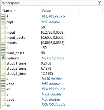
Study1_time - 9.2168

Study2_time - 6.1878

Study3_time - 12.1395

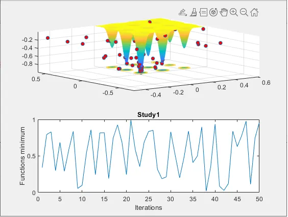
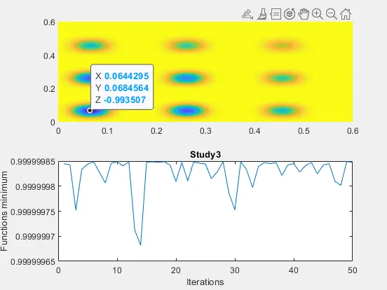
PLOT GRAPH – STUDY 1

According to study 1 we can see that we have ploted the stalagmite function. The x axis consist of the iterations starting from 0 to 50 and the y axis consist of the functions minimum starting from 0 to 1. So we can see the values changes from zero to 1 in the graph.

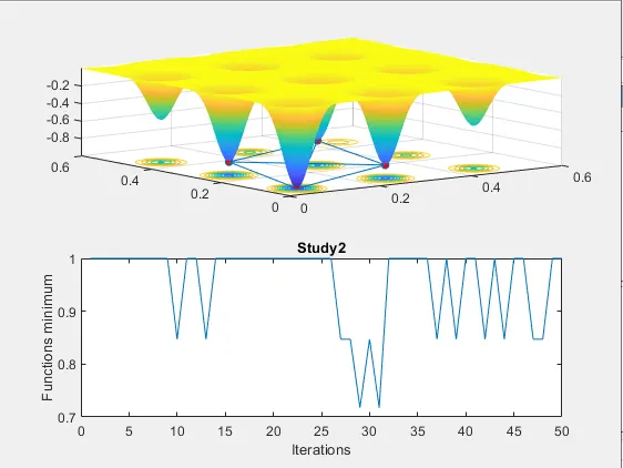
PLOT GRAPH – STUDY 2

In Study 2 we can see that the minimum value is between 0.8 and 0.9

PLOT GRAPH – STUDY 3

In Study 3 we can see that the minimum value is around 0.9

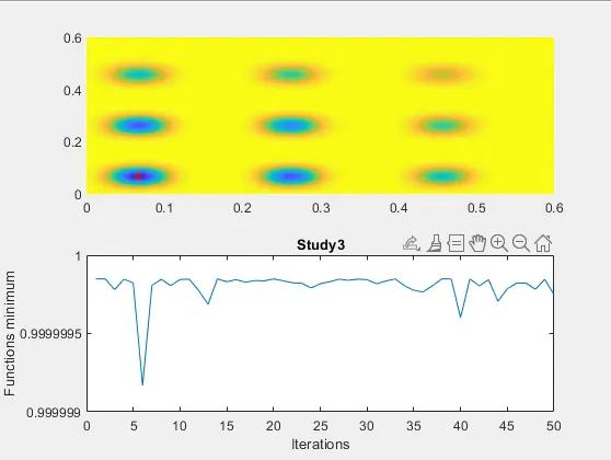
The global minimum and maximum value of x and y is shown below plot graph of Study 3

i.e. X = 0.0644 and Y = 0.0684

SCRIPT WINDOW - Genetic Algorithm

close all
clear all
clc

% Defining our search space
x = linspace(0,0.6,150);
y = linspace(0,0.6,150);
num_cases = 50;

% Creating a 2D mesh
[xx ,yy] = meshgrid(x,y);

% Evaluating the stalagmite function
for i = 1:length(xx)
    for j = 1:length(yy)
        input_vector(1)=xx(i,j);
        input_vector(2)=yy(i,j);
        f(i,j) = stalagmite_fun(input_vector);
    end
end

tic
% Study 1 - Statistical behavior
for i=1:num_cases
[input,fopt(i)]=ga(@stalagmite_fun,2);
xopt(i)=input(1);
yopt(i)=input(2);
end

study1_time = toc;

figure(1)
subplot(2,1,1)
surfc(xx,yy,f)
hold on
plot3(xopt,yopt,fopt,'o','markersize',5,'markerfacecolor','r')
shading interp
subplot(2,1,2)
plot(-fopt)
xlabel('Iterations')
ylabel('Functions minimum')
title('Study1')
% 
tic
% Study 2 - Statistical behavior - with upper and lower bounds
for i = 1:num_cases
    [inputs, fopt(i)] = ga(@stalagmite_fun,2,[],[],[],[],[0;0],[0.6,0.6]);
    xopt(i) = inputs(1);
    yopt(i) = inputs(2);
end
study2_time = toc

figure(2)
subplot(2,1,1)
surfc(xx,yy,f)
hold on
plot3(xopt,yopt,fopt,'marker','o','markersize',5,'markerfacecolor','r')
shading interp
subplot(2,1,2)
plot(-fopt)
xlabel('Iterations')
ylabel('Functions minimum')
title('Study2')

% Study 3 increasing GA iterations
options = optimoptions('ga');
options = optimoptions(options,'PopulationSize', 170);

tic
for i = 1:num_cases
    [inputs, fopt(i)] = ga(@stalagmite_fun,2,[],[],[],[],[0;0],[0.1,0.1],[],[],options);
    xopt(i) = inputs(1);
    yopt(i) = inputs(2);
end
study3_time = toc


figure(3)
subplot(2,1,1)
hold on
surfc(xx,yy,f)
shading interp
plot3(xopt,yopt,fopt,'marker','o','markersize',5,'markerfacecolor','r')
subplot(2,1,2)
plot(-fopt)
xlabel('Iterations')
ylabel('Functions minimum')
title('Study3')

WORKSPACE

SCRIPT WINDOW - Stalagmite Function

Equation used

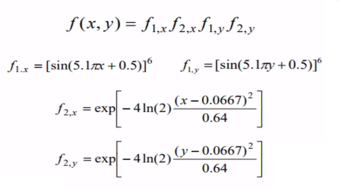
function [f] = stalagmite_fun(input_vector)

x=input_vector(1);
y=input_vector(2);
f1=(sin((5.1*pi*x+0.5)))^6;
f2=((sin(5.1*pi*y+0.5)))^6;
f3= exp((-4*log(2)*((x-0.0667)^2)/0.64));
f4=exp((-4*log(2)*((y-0.0667)^2)/0.64));
f=(f1*f2*f3*f4*-1);



end

ERROR

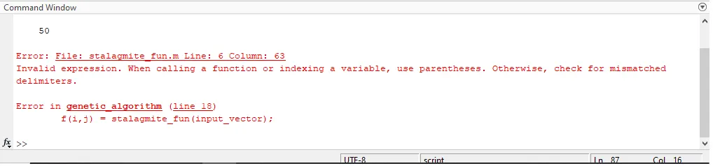
The below error showed up when i had a repeated typo error in yopt as ypot, stalagmite function name and the function command in stalagmite function had paranthesis usage error result in error line18.