Week 4 - Genetic Algorithm

Aim:

To write a code in MATLAB to optimize the stalagmite function and find the global maxima of the function.

Concept of Genetic Algorithm:

A Genetic Algorithm is a search and divide technique that is inspired by Charles Darwin’s theory of natural evolution which basically does the process of natural selection where the fittest individuals are selected for reproduction in order to produce offspring of the next generation. In this way, the offspring would be best and the fittest.

Five phases are considered in a genetic algorithm.

1. Initial population
2. Fitness function
3. Selection
4. Crossover
5. Mutation

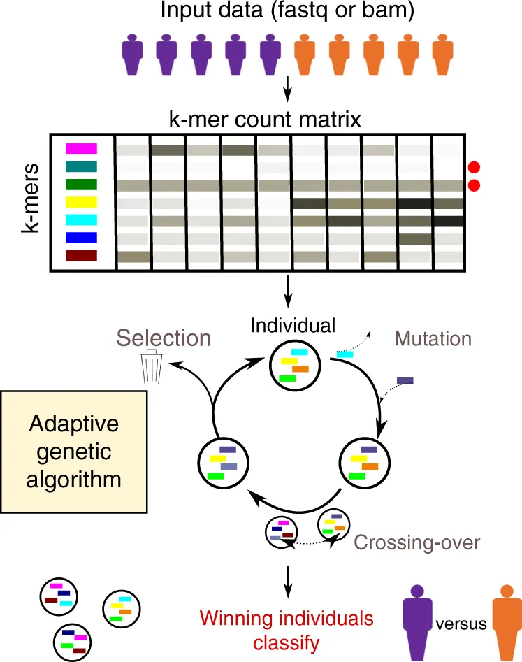
For Detailed Information You can go through the following reference:

https://towardsdatascience.com/introduction-to-genetic-algorithms-including-example-code-e396e98d8bf3#:~:text=A%20genetic%20algorithm%20is%20a,offspring%20of%20the%20next%20generation.

Now for the Program following Formula has been taken into consideration

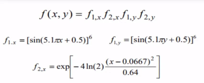
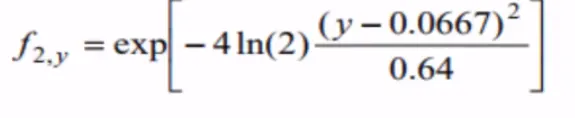
Program 1: Now Function for Stalagmite is as follows based on the above formula

function[f]=stalagmite(input_vector)

x=input_vector(1);
y=input_vector(2);

ax=(sin(5.1*pi*x+0.5))^6;
ay=(sin(5.1*pi*y+0.5))^6;
bx=exp(-4*log(2)*((x-0.0667)^2/0.64));
by=exp(-4*log(2)*((y-0.0667)^2/0.64));
f=-(ax*bx*ay*by);
end

Explanation of Program:

Steps:

1. The function is declared with the name Stalagmite
2. Two inputs variables (x and y) are considered
3. Based on the above formula each individual polynomial is taken into the account name ax, ay, bx & by
4. Finally the -ve sign has been put optimize stability for the Ga function (taking minimum value in the account)

ga or Genetic Algorithm syntax explanation:

1. What does ga do?

x = ga(fun,nvars) finds a local unconstrained minimum, x, to the objective function, fun. nvars is the dimension (number of design variables) of function.

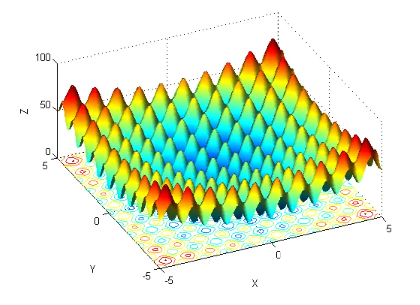
For Example, This is one of the Plots showing the global minimum:

Program 2: Main Program to find the global maximum value:

clear all
close all
clc

% Defining the Search Space
x = linspace(0,0.6,150);
y = linspace(0,0.6,150);
num_cases=50
% Creating a 2d dimensional mesh
[xx, yy] = meshgrid(x,y);
% Evaluating the stalagamite Function

for i=1:length(xx)
    for j=1:length(yy)
        input_vector(1)=xx(i,j);
        input_vector(2)=yy(i,j);
        f(i,j)= stalagmite(input_vector);
    end
end

tic

for i= 1:num_cases
    [inputs,fopt(i)]=ga(@stalagmite,2);
    xopt(i)=inputs(1);
    yopt(i)=inputs(2);
end
study_time=toc

figure(1)
subplot(2,1,1)
hold on
surfc(x,y,-f)
shading interp
plot3(xopt,yopt,-fopt,'marker','o','markersize',10,'markerfacecolor','r')
title('Unbounded Inputs')
subplot(2,1,2)
plot(-fopt)
xlabel('Iterations')
ylabel('Fuction Maximum')


%Study2 statistics
tic

for i= 1:num_cases
    [inputs,fopt(i)]=ga(@stalagmite,2,[],[],[],[],[0;0],[0.6;0.6]);
    xopt(i)=inputs(1);
    yopt(i)=inputs(2);
end
study2_time=toc

figure(2)
subplot(2,1,1)
hold on
surfc(x,y,-f)
shading interp
plot3(xopt,yopt,-fopt,'marker','o','markersize',10,'markerfacecolor','r')
title('Bounded Inputs')
subplot(2,1,2)
plot(-fopt)
xlabel('Iterations')
ylabel('Fuction Maximum')

%Study3 statistics

options=optimoptions('ga');
options=optimoptions(options,'PopulationSize',150);
tic

for i= 1:num_cases
    [inputs,fopt(i)]=ga(@stalagmite,2,[],[],[],[],[0;0],[1;1],[],[],options);
    xopt(i)=inputs(1);
    yopt(i)=inputs(2);
end
study3_time=toc

figure(3)
subplot(2,1,1)
surfc(x,y,-f)
shading interp
hold on
plot3(xopt,yopt,-fopt,'marker','o','markersize',10,'markerfacecolor','r')
title('Bounded Inputs')
subplot(2,1,2)
plot(-fopt)
xlabel('Iterations')
ylabel('Fuction Minimum')






        

Explanations of the Program 2

Steps

1. The general search space has been defined between 0 to 0.6
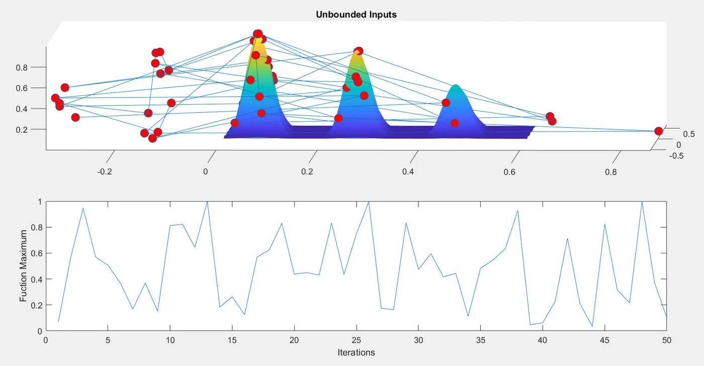
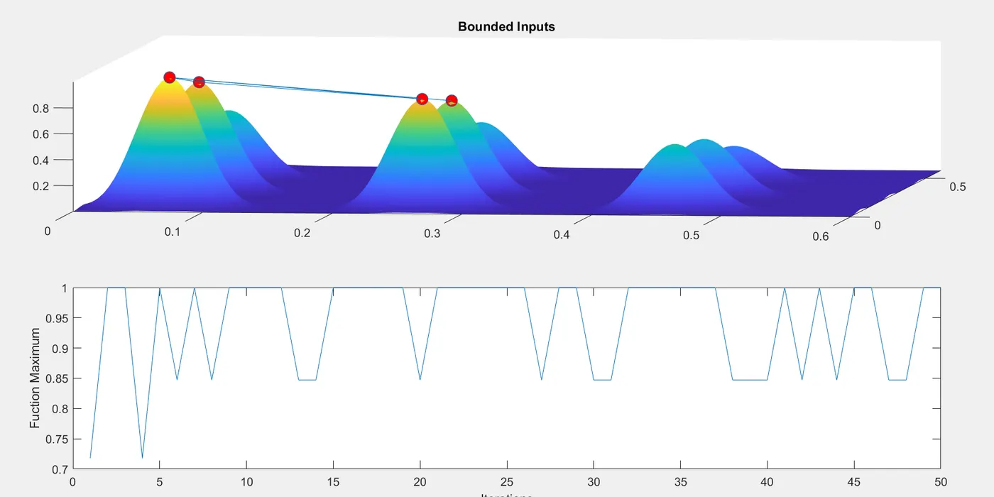
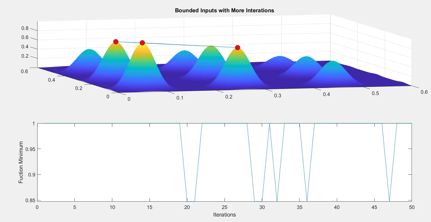
2. The Red pointers (shown in the graph below) are node points confined within the search brackets
3. The stalagmite function is being called to find and optimize the given function
4. The graph is set (surfc) command is used for the shaded and Mountain representations of the peak values
5. The ga function is now used to find the global maximum value in the function
6. Important: Here as shown in the program the f output is kept in -ve, this is because Ga peaks the minimum value which is difficult to peak in the already negative function thus by putting the -ve sign we are reversing the graph plotting so as to get the maximum value easily from the +ve output
7. With three statistics involved the increasing number of iterations gives the output

Graph Results and Output Plot of the program:

Graph 1 statistical 1

Graph 2 statistical 2

Graph 3 statistical 3

Conclusion:

Thus the program for finding the global maxima value for the given function is created and increasing the number of iterations is decreasing the search space for the right value also the ga function is utilized and made to understand by providing necessary examples