Genetic Algorithm
Genetic Algorithm
Aim: Writing a program in MATLAB to optimise the stalagmite function and find the global maxima of the function.
Objective:
- Optimise stalagmite function.
- Finding the global maxima.
- Plotting graph for 3 studies and for F maximum v/s no. of iterations.
Methodology:
Theory
Genetic Algorithm
The genetic algorithm is a method for solving both constrained and unconstrained optimization problems that is based on natural selection, the process that drives biological evolution. The genetic algorithm repeatedly modifies a population of individual solutions. At each step, the genetic algorithm selects individuals at random from the current population to be parents and uses them to produce the children for the next generation. Over successive generations, the population "evolves" toward an optimal solution. You can apply the genetic algorithm to solve a variety of optimization problems that are not well suited for standard optimization algorithms, including problems in which the objective function is discontinuous, nondifferentiable, stochastic, or highly nonlinear. The genetic algorithm can address problems of mixed integer programming, where some components are restricted to be integer-valued.
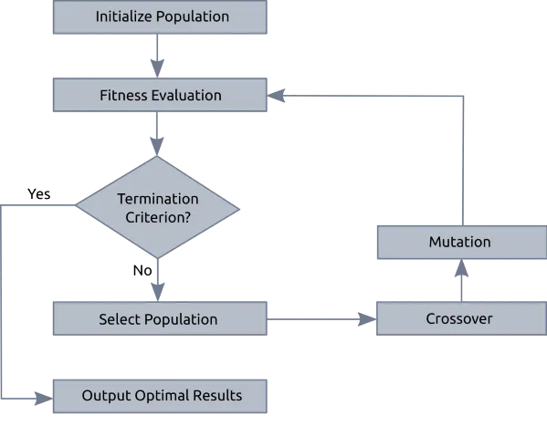
Fig: Basic Structure of Genetic Algorithm
The genetic algorithm creates three types of children for the next generation:
-
Elite are the individuals in the current generation with the best fitness values. These individuals automatically survive to the next generation.
-
Crossover are created by combining the vectors of a pair of parents.
-
Mutation children are created by introducing random changes, or mutations, to a single parent.
The following schematic diagram illustrates the three types of children.
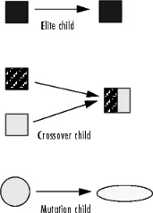
Fig: Types of Children
The genetic algorithm differs from a classical, derivative-based, optimization algorithm in two main ways, as summarized in the following table.
| Classical Algorithm | Genetic Algorithm |
|---|---|
|
Generates a single point at each iteration. The sequence of points approaches an optimal solution. |
Generates a population of points at each iteration. The best point in the population approaches an optimal solution. |
|
Selects the next point in the sequence by a deterministic computation. |
Selects the next population by computation which uses random number generators. |
Optimization
Optimization is the process of making something better. In any process, we have a set of inputs and a set of outputs as shown in the following figure.
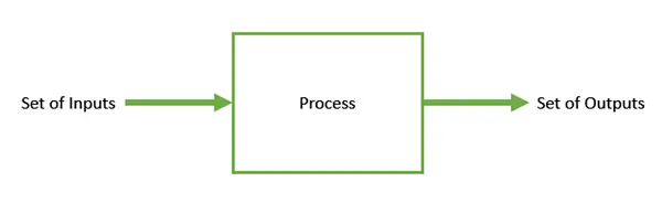
Fig: Optimization Block Diagram
Optimization refers to finding the values of inputs in such a way that we get the “best” output values. The definition of “best” varies from problem to problem, but in mathematical terms, it refers to maximizing or minimizing one or more objective functions, by varying the input parameters.
The set of all possible solutions or values which the inputs can take make up the search space. In this search space, lies a point or a set of points which gives the optimal solution. The aim of optimization is to find that point or set of points in the search space.
Nature has always been a great source of inspiration to all mankind. Genetic Algorithms (GAs) are search based algorithms based on the concepts of natural selection and genetics. GAs are a subset of a much larger branch of computation known as Evolutionary Computation.
GAs were developed by John Holland and his students and colleagues at the University of Michigan, most notably David E. Goldberg and has since been tried on various optimization problems with a high degree of success.
Foundation of Genetic Algorithm
Genetic algorithms are based on an analogy with genetic structure and behavior of chromosome of the population. Following is the foundation of GAs based on this analogy –
- Individual in population compete for resources and mate
- Those individuals who are successful (fittest) then mate to create more offspring than others
- Genes from “fittest” parent propagate throughout the generation, that is sometimes parents create offspring which is better than either parent.
- Thus each successive generation is more suited for their environment.
In GAs, we have a pool or a population of possible solutions to the given problem. These solutions then undergo recombination and mutation (like in natural genetics), producing new children, and the process is repeated over various generations. Each individual (or candidate solution) is assigned a fitness value (based on its objective function value) and the fitter individuals are given a higher chance to mate and yield more “fitter” individuals. This is in line with the Darwinian Theory of “Survival of the Fittest”.
In this way we keep “evolving” better individuals or solutions over generations, till we reach a stopping criterion.
Genetic Algorithms are sufficiently randomized in nature, but they perform much better than random local search (in which we just try various random solutions, keeping track of the best so far), as they exploit historical information as well.
Advantages of GAs
GAs have various advantages which have made them immensely popular. These include −
-
Does not require any derivative information (which may not be available for many real-world problems).
-
Is faster and more efficient as compared to the traditional methods.
-
Has very good parallel capabilities.
-
Optimizes both continuous and discrete functions and also multi-objective problems.
-
Provides a list of “good” solutions and not just a single solution.
-
Always gets an answer to the problem, which gets better over the time.
-
Useful when the search space is very large and there are a large number of parameters involved.
Limitation of GAs
Like any technique, GAs also suffer from a few limitations. These include −
-
GAs are not suited for all problems, especially problems which are simple and for which derivative information is available.
-
Fitness value is calculated repeatedly which might be computationally expensive for some problems.
-
Being stochastic, there are no guarantees on the optimality or the quality of the solution.
-
If not implemented properly, the GA may not converge to the optimal solution.
Genetic Algorithms have the ability to deliver a “good-enough” solution “fast-enough”. This makes genetic algorithms attractive for use in solving optimization problems. The reasons why GAs are needed are as follows −
In computer science, there is a large set of problems, which are hard. What this essentially means is that, even the most powerful computing systems take a very long time to solve that problem. In such a scenario, GAs prove to be an efficient tool to provide usable near-optimal solutions in a short amount of time.
Traditional calculus based methods work by starting at a random point and by moving in the direction of the gradient, till we reach the top of the hill. This technique is efficient and works very well for single-peaked objective functions like the cost function in linear regression. But, in most real-world situations, we have a very complex problem called as landscapes, which are made of many peaks and many valleys, which causes such methods to fail, as they suffer from an inherent tendency of getting stuck at the local optima as shown in the following figure.
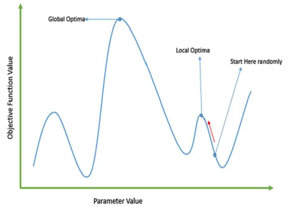
Fig: Global Maxima on a graph
Operators of Genetic Algorithm
Once the initial generation is created, the algorithm evolve the generation using following operators –
1) Selection Operator: The idea is to give preference to the individuals with good fitness scores and allow them to pass there genes to the successive generations.
2) Crossover Operator: This represents mating between individuals. Two individuals are selected using selection operator and crossover sites are chosen randomly. Then the genes at these crossover sites are exchanged thus creating a completely new individual (offspring). For example –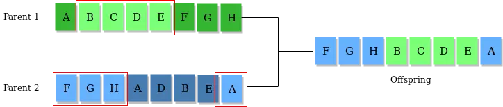
Fig: Selection and Crossover
3) Mutation Operator: The key idea is to insert random genes in offspring to maintain the diversity in population to avoid the premature convergence. For example –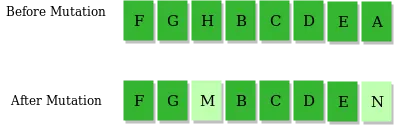
Fig: Mutation
MATLAB Program
Stalagmite Function
The relation of stalagmite function for global minima is given as;
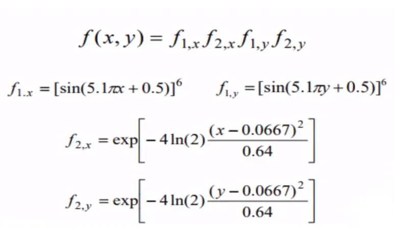
Fig: Equation of stalagmite function for Global Minima
From the above equations, we can create the function of stalagmite.
But, with the above mentioned formula, we can find the global minima. To find global maxima there is a small spin to it.
function [f] = popstalagmite(input_vector)
x = input_vector(1);
y = input_vector(2);
f1x = (sin((5*pi*x)+0.5))^6;
f1y = (sin((5*pi*y)+0.5))^6;
f2x = exp(((-4*log(2))*((x-0.0667)^2))/(0.64));
f2y = exp(((-4*log(2))*((y-0.0667)^2))/(0.64));
[f] = -(f1x*f2x*f1y*f2y);                      %Global Maxima

% B = f^-1;
% C= (1/(1+f));
end
In the main program, we will will to input vector that goes to function. Here the function takes those two values and we assign those values to variable 'x' and 'y'. Once both the variable are stored, we can now now find the f1x, f1y, f2x and f2y . Now we do the multiplication of all these four variable which gives the global minima. What we can essentially do is convert this into global maxima. To do this, we have 3 ways. The are as follow;
1. Changing the sign of the 'f' after the multiplication is done.
2. Doing the inverse of the 'f'.
3. Using the relation (1/1+f).
But, choosing of the method is not random. First we find the global maxima using all three ways, then we compare the result of all all three. The method that yield highest result of global maxima is chosen. In this application, the changing of the sign of 'f' is done, as it yielded the highest result.
Main Program
%A Program to find Global Maxima for a given population size
clear all
close all
clc

%Input
x = linspace(0,0.6,150);                                   %Upper and lower bound on X Co-ordinate
y = linspace(0,0.6,150);                                   %Upper and lower bound on Y Co-ordinate
num_case = input('Enter the default Number of cases:');    %User input on default cases
l = input('Enter the Final Population Size:');             %User input on final sample size
%Creating 2D array
[xx yy] = meshgrid(x,y);

%Evaluating the stalagmite function
for i = 1:length(xx)
    for j = 1:length(yy)
        input_vector(1) = xx(i,j);
        input_vector(2) = yy(i,j);
        f(i,j) = popstalagmite(input_vector);              %Every possible values generation
    end
end

tic
%Study 1 - Statistical Behaviour
for  i = 1:num_case
    [inputs, fopt(i)] = ga(@popstalagmite,2);
    xopt(i) = inputs(1);
    yopt(i) = inputs(2);
end
figure(1)
subplot(2,1,1)
hold on
surfc(xx,yy,-f)                                            %Surface generation
shading interp                                             %Removing Mesh grid from surface
plot3(xopt,yopt,-fopt,'marker','o','markersize',5,'markerfacecolor','r')
title('Unbounded Inputs')
xlabel('xx')
ylabel('yy')
zlabel('-f')
subplot(2,1,2)
plot(-fopt)
xlabel('Iterations')
ylabel('Function Maximum')
study1_time = toc

tic
%Study 2 - Statistical Behaviour - with upper and lower bounds
for  i = 1:num_case
    [inputs, fopt(i)] = ga(@popstalagmite,2,[],[],[],[],[0;0],[0.6;0.6]);
    xopt(i) = inputs(1);
    yopt(i) = inputs(2);
end
figure(2)
subplot(2,1,1)
hold on
surfc(xx,yy,-f)                                            %Surface generation
shading interp                                             %Removing Mesh grid from surface
plot3(xopt,yopt,-fopt,'marker','o','markersize',5,'markerfacecolor','r')
title('Unbounded Inputs')
xlabel('xx')
ylabel('yy')
zlabel('-f')
subplot(2,1,2)
plot(-fopt)
xlabel('Iterations')
ylabel('Function Maximum')
study2_time = toc

tic
%Study 3 - Statistical Behaviour -Increasing GA Iterations
options = optimoptions('ga');
options = optimoptions(options,'PopulationSize',l);

for  i = 1:num_case
    [inputs, fopt(i)] = ga(@popstalagmite,2,[],[],[],[],[0;0],[0.6;0.6],[],[],options);
    xopt(i) = inputs(1);
    yopt(i) = inputs(2);
end
figure(3)
subplot(2,1,1)
hold on
surfc(xx,yy,-f)                                            %Surface generation
shading interp                                             %Removing Mesh grid from surface
plot3(xopt,yopt,-fopt,'marker','o','markersize',5,'markerfacecolor','r')
title('Unbounded Inputs')
xlabel('xx')
ylabel('yy')
zlabel('-f')
subplot(2,1,2)
plot(-fopt)
xlabel('Iterations')
ylabel('Function Maximum')
study3_time = toc
We as usual began our coding by clearing workspace window and command window.
Here, first we need to create every number of possiblity for the given sample. What we essentially do is create the inpute. We create variable 'x' and 'y' and using linspace command create 150 values between 0 and 0.6. Using 0.6, we do know that we will get 9 different area on our stalagmite function.
The number of default cases (num_case) can be given as a user input or can be set to default. I have given a user input. The same can be said about the final smaple size (l). The num_case we used is 50 and increased size is 170 to get the better result in determining Global Maxima
We the create a 2D array of vaiable x and y using the function meshgrid and store them in variable xx and yy.
Creating every possible result
The first for loop, takes the length of xx as the number of time it will iterate and the nested for loop take the length of yy. For every point of xx and yy, we get every possible result. First the value of xx(i,j) is stored in variable input_vector(1) and yy(i,j) is stored in input_vector(2). The next step send this value to the function popstalagmite and return the value of 'f' in f(i,j). This thing will produce 22,500 results.
Study Case 1
In this study, we find out the statistical behaviour of the result.
We have made use of tic and toc command to find out time of iteration and determining result. The tic starts the clock and toc stops the clock time, the clock time stored in toc is stored in study1_time.
From programming point of view, we use the for loop, that will run until the number of default cases (num_case). We set the output using 'ga' function in [inputs and fopt(i)].
The syntax used here is:
x = ga(fun,nvars);
For generatic algorithm, which means first we mention the function, where it will perform the operation and return the value, in our case the function is popstalagmite. And the number of design variables is nvars, which in our case is 2. So we give input as;
ga(stalagmite,2);
The returned two value is stored in xopt and yopt.
Once all the values are stored, we plot a graph based on this values. Mentioning figure(1), we are creating two subplot (2,1,1) and (2,1,2). Using hold on command the plot is held and the next plot will be created on the same graph. Using surfc command, what we are doing is creating the graph of co-ordinate xx,yy and -f. The sign is minus to give us the result in positive co-ordinates.
shading interp is used to actually avoid the mesh grid on the result, what is does is makes the result better for illustration. Next using plot 3 command we can plot graph of 3 axis, here the axis are xopt, yopt and -fopt. Again to get the result in positive co-ordinates. We also select the specification of plot, where the main point is shown using 'marker' 'o', 'markersize' is set at '5' and 'markercolor' is given as 'r' (red). Using title command we give title to our graph as "Unbounded Inputs", using label we name X co-ordinate as xx, Y co-ordinate as yy, and Z co-ordinate as -f. In second subplot, we plot '-fopt'. Using label we will name X co-ordinate as 'Iterations' and Y co-ordinate as 'Function Maximum'.
Study Case 2
In this study, we find out the statistical behaviour of the result by giving upper and lower bounds.
We have made use of tic and toc command to find out time of iteration and determining result. The tic starts the clock and toc stops the clock time, the clock time stored in toc is stored in study2_time.
From programming point of view, we use the for loop, that will run until the number of default cases (num_case). We set the output using 'ga' function in [inputs and fopt(i)].
The syntax used here is:
x = ga(fun,nvars,A,b,Aeq,beq,lb,ub)
For generatic algorithm, which means first we mention the function, where it will perform the operation and return the value, in our case the function is popstalagmite. And the number of design variables is nvars, which in our case is 2. Incase of no linear inequalities, A, B, Aeq and Beq is []. Our lower limit for X and Y co-ordinate is 0. Our upper limit of X as well as Y co-ordinate is 0.6. So we give input as;
ga(@popstalagmite,2,[],[],[],[],[0;0],[0.6;0.6]);
The returned two value is stored in xopt and yopt.
Once all the values are stored, we plot a graph based on this values. Mentioning figure(1), we are creating two subplot (2,1,1) and (2,1,2). Using hold on command the plot is held and the next plot will be created on the same graph. Using surfc command, what we are doing is creating the graph of co-ordinate xx,yy and -f. The sign is minus to give us the result in positive co-ordinates.
shading interp is used to actually avoid the mesh grid on the result, what is does is makes the result better for illustration. Next using plot 3 command we can plot graph of 3 axis, here the axis are xopt, yopt and -fopt. Again to get the result in positive co-ordinates. We also select the specification of plot, where the main point is shown using 'marker' 'o', 'markersize' is set at '5' and 'markercolor' is given as 'r' (red). Using title command we give title to our graph as "Unbounded Inputs", using label we name X co-ordinate as xx, Y co-ordinate as yy, and Z co-ordinate as -f. In second subplot, we plot '-fopt'. Using label we will name X co-ordinate as 'Iterations' and Y co-ordinate as 'Function Maximum'.
Study Case 3
In this study, we find out the statistical behaviour of the result by increasing the GA iteration as well as optimising GA
We have made use of tic and toc command to find out time of iteration and determining result. The tic starts the clock and toc stops the clock time, the clock time stored in toc is stored in study3_time.
Using the syntax, options = optimoptions(SolverName), returns a set of default options for the SolverName solver. In our case, it is 'ga'
options = optimoptions('ga');
Using the syntax, options = optimoptions(SolverName,Name,Value), returns options with the named parameters altered with the specified values. In our case, tha name is PopulationSize, which will take user defined input in variable 'l'.
options = optimoptions(options,'PopulationSize',l);
We will Population Size as 170, as it gives better result while determining Global Maxima.
From programming point of view, we use the for loop, that will run until the number of default cases (num_case). We set the output using 'ga' function in [inputs and fopt(i)].
The syntax used here is:
x = ga(fun,nvars,A,b,Aeq,beq,lb,ub,nonlcon,options)
For generatic algorithm, which means first we mention the function, where it will perform the operation and return the value, in our case the function is popstalagmite. And the number of design variables is nvars, which in our case is 2. Incase of no linear inequalities, A, B, Aeq and Beq is []. Our lower limit for X and Y co-ordinate is 0. Our upper limit of X as well as Y co-ordinate is 0.6. nonlcon=[] because there no nonlinear constraints. We have created options using optimoptions, which will give optimised result. So we give input as;
ga(@popstalagmite,2,[],[],[],[],[0;0],[0.6;0.6],[],[],options);
The returned two value is stored in xopt and yopt.
Once all the values are stored, we plot a graph based on this values. Mentioning figure(1), we are creating two subplot (2,1,1) and (2,1,2). Using hold on command the plot is held and the next plot will be created on the same graph. Using surfc command, what we are doing is creating the graph of co-ordinate xx,yy and -f. The sign is minus to give us the result in positive co-ordinates.
shading interp is used to actually avoid the mesh grid on the result, what is does is makes the result better for illustration. Next using plot 3 command we can plot graph of 3 axis, here the axis are xopt, yopt and -fopt. Again to get the result in positive co-ordinates. We also select the specification of plot, where the main point is shown using 'marker' 'o', 'markersize' is set at '5' and 'markercolor' is given as 'r' (red). Using title command we give title to our graph as "Unbounded Inputs", using label we name X co-ordinate as xx, Y co-ordinate as yy, and Z co-ordinate as -f. In second subplot, we plot '-fopt'. Using label we will name X co-ordinate as 'Iterations' and Y co-ordinate as 'Function Maximum'.
Stopping Criteria
It is known that iterative solutions to problems improve initially but deteriorate after some point. This highlights the importance of knowing when it is time to stop. It will not necessarily deteriorate, sometimes the result will remain the same and the iteration goes on and on. In the termination condition of a Genetic Algorithm, it has been observed that initially, the GA progresses very fast with better solutions coming in every few iterations, but this tends to saturate in the later stages where the improvements are very small. We usually want a termination condition such that our solution is close to the optimal, at the end of the run.
Usually, we keep one of the following termination conditions −
- When there has been no improvement in the population for X iterations.
- When we reach an absolute number of generations.
- When the objective function value has reached a certain pre-defined value.
Stopping Condition for Genetic Algorithm
The genetic algorithm uses the following options to determine when to stop. See the default values for each option by running opts = optimoptions('ga').
- MaxGenerations — The algorithm stops when the number of generations reaches MaxGenerations.
- MaxTime — The algorithm stops after running for an amount of time in seconds equal to MaxTime.
- FitnessLimit — The algorithm stops when the value of the fitness function for the best point in the current population is less than or equal to FitnessLimit.
- MaxStallGenerations — The algorithm stops when the average relative change in the fitness function value over MaxStallGenerations is less than Function tolerance.
- MaxStallTime — The algorithm stops if there is no improvement in the objective function during an interval of time in seconds equal to MaxStallTime.
- FunctionTolerance — The algorithm runs until the average relative change in the fitness function value over MaxStallGenerations is less than Function tolerance.
- ConstraintTolerance — The ConstraintTolerance is not used as stopping criterion. It is used to determine the feasibility with respect to nonlinear constraints. Also, max(sqrt(eps),ConstraintTolerance) determines feasibility with respect to linear constraints.
The algorithm stops as soon as any one of these conditions is met.
Significance of running multiple iterations
Algorithms consist of steps that are carried out one after another. Sometimes an algorithm needs to repeat certain steps until told to stop or until a particular condition has been met. Iteration allows us to simplify our algorithm by stating that we will repeat certain steps until told otherwise.
Its significance in GA can be clearly understood by the fact that, in GA we create as many possiblities we can at first. The iteration helps us to create all of the possiblities in a short span and without repeating the code.
The significance in terms of getting the best result in GA can be found out by increasing the number of studies. The increase in the number of studies gives the result better. In our case, we did 3 studies where in first study we got many points on the graph as maxima. But in second iteration, by giving bound constraints we got selected number of points where the result would lie. But during the next iteration, while optimising we get the exact point of maxima. Sometimes, we may not get the single point, it maybe multiple result from which the maxima will be one. In that case, the maxima can be achieved by doing another study. In this case, 'Global Maxima' was achieved after 3 studies.
In Matrices, iterative step do result in converged and better result in every step. But that result do need a termination after certain point. When all the conditions are met, the algorithm stops.
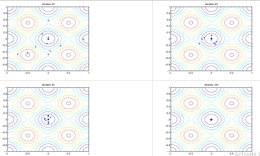
Fig: Iterative result
The above figure shows the populations at iterations 60, 80, 95, and 100. At every iteration, the result converges and gives better result. Once are condition is met of finding 'Global Maxima', the iteraration is stopped.
Result:
Study 1
In study 1, we see that the plots has list of scattered point, with no clear Global Maxima Point. This is also called as point where we have result for Population Size. The graph of Iterations against maximu does not clearly indicate the maximum point. The graph can be seen as below;
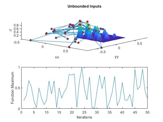
Fig: Statistical Behaviour
The study1_time is 4.5654 sec.
Study 2
In study 2, we have set the upper and lower limit as well as have set the inequalities to []. What this does is give set of few points where the maxima will be located. The graph of Iterations against Function Maximum will give clear set of point on a graph where maxima will be located. This step is also called as Bound Constraints. The graph can be seen as below;
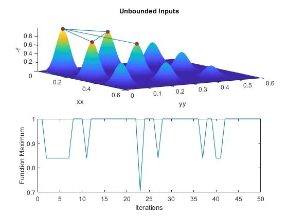
Fig: Statistical Behaviour with upper and lower bound
The study2_time is 5.6809 sec.
Study 3
In study 3, we have set the optimisation of 'ga', upper and lower limit, set the inequalities to []. What this does is give exact point where the maxima will be located. The graph of Iterations against Function Maximum will clearly give the point on a graph where maxima will be located. This step is also called as Optimisation. The graph can be seen as below;
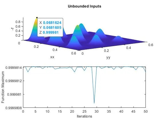
Fig: Statistical Behaviour during optimisation and increasing GA iteration
The study3_time is 14.8682 sec.
The 'Global Maxima' is 0.999981 located at (0.0682,0.0682).
Learning Outcome:
- Understood the basic of Genetic Algorithm.
- Learned and implemented 'ga' function.
- Learned and implemented stalagmite function.
- Learned method to optimise 'Global Maxima'.
- Learned to create 3 dimensional plot.
Conclusion:
Created a MATLAB program to optimise the stalagmite function and find the global maxima of the function. Also plotted the graph for all 3 studies and for Iterations against Function Maximum.
References:
- https://in.mathworks.com/help/gads/what-is-the-genetic-algorithm.html
- https://www.tutorialspoint.com/genetic_algorithms/genetic_algorithms_introduction.htm
- https://www.tutorialspoint.com/genetic_algorithms/genetic_algorithms_termination_condition.htm
- https://in.mathworks.com/help/gads/how-the-genetic-algorithm-works.html