Week 4 - Genetic Algorithm

AIM : To write code in matlab to optimize stalagmite function and find global maxima.

OPTIMISATION : Optimisation is a decision making process. Optimisation is important to get best results which includes adding or lowering a value in a sysem. This helps us to get a better efficiency and reliability of a system.

GENETIC ALGORITHM : It is an optimisation technique which works on the principle of Charles Darwin's genetics and natural selection.

There are three processes involved in genetic algorithm ,

*SELECTION - Here parents are selected from a sample data. Highly fit individuals are selected. The features of parents are transmitted to next generation.

*CROSS OVER - After selection , the features of parents are drawn and they are combined to produce a new offspring.

*MUTATION - This is carried out to obtain diversity and similar genes could result in local minima.

STALAGMITE : It is a type of rock that rises from floor to ceiling or vice versa that is formed due to the accumalation of materials deposited.

It is used in GA as a function to optimze values and helps to understand about the maxima and minimum values through its representation.

CODE :

(1) clear all,close all and clc is used to close variables,plots and command window respectively.

(2) Linspace is used represent variables in array format and here 0-0.6 value is set as minimum and maximum and number of elements is given as 150 which means 150 values are present between 0-0.6.

(3) Input value of 60 is assigned to a variable num_case.

(4) meshgrid command is used to make 2D grids on given co-ordinates.

(5) Declaration of i and j is made. In the case 1 command [input,fopt(i)]=ga(@stalagmite,2) is used under for loop to carry out first process where unbounded random number of maximum values are selected.

(6) GA is used to find global minimum. To find global maximum , we have to use negative (-) value for f so that the direction of values are reversed.

(7)surfc command is used to create a 3D representation. xlabel and ylabel are used to denote and label what we have assigned.

(8) shading interp is used to give provide a smoother representation.

(9) The first figure represents the stalagmite function and the second represents the values that lie within the function range with respect to iterations.

(10) In case 2 and 3 , we start to do optimization and we find maxima. There is a similarity of code with case 1 but we need to change syntax of genetic algorithm.

x = ga(@stalagmite,nvars,a,b,aeq,beq,lb,ub)

where x is the variable which stores the value, nvars is number of variables , a and b are linear inequality constraints , aeq and beq are linear equality constraints , lb and ub are lower and upper bounds respectively. This generates values that are bounded and helps to increase accuracy.

(11) In case 3 ,

options=optimoptions('ga');
options=optimoptions(options,'populationsize',100) is used which optimizes the values to give us more accurate maximum value. population size is increased here. It can also be further increased to get even better accurate value.

clear all
close all
clc

%defining our search space 
x=linspace(0,0.6,150);
y=linspace(0,0.6,150);
num_case=60;

%creating a 2D mesh
[xx yy]=meshgrid(x,y);

%evaluating stalagmite function
for i = 1:length(xx)
    for j = 1:length(yy)
        input_vector(1)=xx(i,j);
        input_vector(2)=yy(i,j);
        f(i,j) = stalagmite(input_vector);
    end
end

% case 1
tic

for i=1:num_case
    
    [input,fopt(i)]=ga(@stalagmite,2);
    x_opt(i)=input(1);
    y_opt(i)=input(2);
    
end

case_time_1=toc

figure(1)
subplot(2,1,1)
surfc(xx,yy,-f)
xlabel('x')
ylabel('y')
title('case 1','color','k')
shading interp
hold on
plot3(x_opt,y_opt,-fopt,'marker','o','markersize',5,'markerfacecolor','r');
subplot(2,1,2)
plot(-fopt);
xlabel('iterations')
ylabel('function max')

%case 2 

tic
for i=1:num_case
    
    [input,fopt(i)]=ga(@stalagmite,2,[],[],[],[],[0;0],[1;1]);
    x_opt(i)=input(1);
    y_opt(i)=input(2);
end

case_time_2=toc

figure(2)
subplot(2,1,1)
hold on
surfc(xx,yy,-f)
xlabel('x')
ylabel('y')
title('case 2','color','k')
shading interp
plot3(x_opt,y_opt,-fopt,'marker','o','markersize',5,'markerfacecolor','r');
subplot(2,1,2)
plot(-fopt);
xlabel('iterations')
ylabel('function max') 

%case 3

options=optimoptions('ga');
options=optimoptions(options,'populationsize',100)

tic
for i=1:num_case
    
    [input,fopt(i)]=ga(@stalagmite,2,[],[],[],[],[0;0],[1;1],[],[],options);
    x_opt(i)=input(1);
    y_opt(i)=input(2);
end

case_time_3=toc

figure(3)
subplot(2,1,1)
hold on
surfc(xx,yy,-f)
xlabel('x')
ylabel('y')
title('case 3','color','k')
shading interp
plot3(x_opt,y_opt,-fopt,'marker','o','markersize',5,'markerfacecolor','r');
subplot(2,1,2)
plot(-fopt);
xlabel('iterations')
ylabel('function max') 

FUNCTION DEFINITION :

function f = stalagmite(input_vector)
x = input_vector(1);
y = input_vector(2);
f1 = (sin(5.1*pi*x+0.5)).^6;
f2 = exp((-4*log(2)*((x-0.0667).^2))/0.64);
f3 = (sin(5.1*pi*y+0.5)).^6;
f4 = exp((-4*log(2)*((y-0.0667).^2))/0.64);
f5 = (f1*f2*f3*f4);
f=-f5
end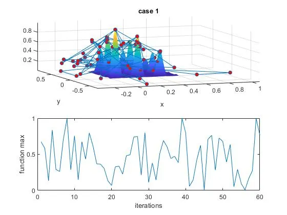

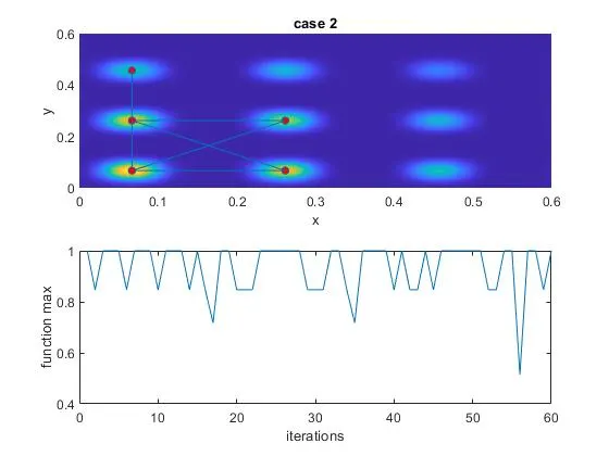
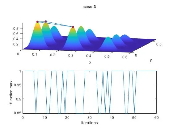
As we could see the values have increased in case 3 to 0.85 compared to case 2.

The values of x and y are 0.06683 & 0.06684 respectively.