Week 4 - Genetic Algorithm

• Write a code in MATLAB to optimise the stalagmite function and find the global maxima of the function.
• Clearly expalin the concept of genetic algorithm in your own words and also explain the syntax for ga in MATLAB in your report.

Theory :

Optimization : Mathematical optimization includes finding 'best available' values of some objective given a defined domain . In the simplest case , an optimization problem consists of maximizing or minimizing a real function by systematically choosing input values from within an allowed set and computing the value of the function. It has applications in many diverse fields suh as engineering , economics,finance, geophysics, molecular modelling, machine learning,etc The ga algorithm always finds the minimum of a function.

An optimization algorithm is a procedure which is executed iteratively by comparing various solutions till an optimum or a satisfactory solution is found. The genetic algorithm is a method for solving both constrained & unconstrained optimization problems that is based on natural selection , the process that drives biological evolution . The genetic algorithm repeatedly modifies a population of individual solutions. At each step , the genetic algorithm selects individuals at random from the current population to be parents & uses them to produce the children for the next generation.Over successive generations, the population "evolves" toward an optimal solution.

Some basic terms of understanding of the working of syntax of the function :

Fitness function : The fitness function is the function to be optimized. For standard optimization algorithms, this is known as objective function .

Individuals : An individual is any point to which you can apply the fitness function, the value of the fitness function for an individual is its score, an individual is sometimes referred to as genome and the vector entries of an individual as genes.

Population & Generations - A population is an array individuals , at each iterations the genetic algorithm performs a series of computations on the current population to produce a new population, each successive population is called a new a generation .

Diversity : Refers to the average distance between individuals in population. A population has high diversity if the average distance is large, diversity is essential to genetic algorithm because it enables the algorithm to search a larger region of space.

Parents & children : To create the next generation , the genetic algorithm selects certain individuals in the current parents , & uses them to create individuals in the next generation called children typically the algorithm is more likely to select parents that have better fittness scores.

Elite children - Are the individuals in the current generation with the best fitness values. these individuals automatically survive to the next generation .

Cross over children : Are created by combining the vectors of a pair of parents.

Mutation children are created by introducing random changes or mutations to s single parent.

The following summarizes how genetic algorithm works :

1) The algorithm begins by creating a random initial population.

2) The algorithm then creates a sequence of new populations, at each step the algorithm uses the individuals in the current generation to create the next population . To create the new population , the algorithm performs the following steps .

• Scores each member of the current population by computing its fitness value , these values are called the raw fitness scores.
• Scores the raw fitness scores to convert them into a more usable range of values. These scaled values are called expectation values. the scaling functions converts the raw fitness scores returned by the fitness function to values in a range that is suitable for the selection function.
• Select the members called parents based on their expectations.
• Some of the individuals in the current populations that have lower fitness (since the algorithm finds the minimum of the fitness function,the best fitness value for a population is the smallest fitness value for any individual in the population) are chosen as elite . These elite individuals are passed to the next population.
• Produces children from the parents , childern are produced either by making randomn changes to s single parent mutation or by combining the vector entries of a pair of parents -cross over.
• Replaces the current population with the children to form the next generation .

3) The algorithm stops when one of the stopping criteria is met , the criteria can be a generation limit a time limit ,fitness limit.

Function Syntax-

[x,fval]= ga(fun,nvars,A,b,Aeq,beq,lb,ub,nonlcon,options)

x--> minimum value of objective function

fval--> Objective function value at the solution

fun--> Fitness function / Objective function

nvars---> number of design variables

A--> Linear inequality contraints, specified as a real matrix. 'A is an M-by-nvars matrix , where m is the number of inqualities

B-->Linear inequality specified as a real vector b is an M element vector related to the A matrix

Aeq-->Linear inequality constraints ,specified as a real vector , Aeq is an Me-by-nvars matrix where Me is the number of equalities.

beq-->Linear inequality constraints, specified as a real vector, beq is an Me-element vector related to the Aeq matrix.

lb-->Bounds the search space of the algorithm.

ub--> Bounds the search space of the algorithm.

nonlcon--> Non linear constriants specified as a function handle or function name.

Options-->Allows us to create plots get data like population size ,sets the limits for algorithm termination.

Function definition of the program

%defining the objective function

function sol = stalagmite(input)

x = input(1);
y = input(2);
f_1_x = (sin(5.1*pi*x+0.5))^6;
f_2_x = exp(-4*(log(2))*(((x-0.0667)^2)/0.64));
f_1_y = (sin(5.1*pi*y+0.5))^6;
f_2_y = exp(-4*(log(2))*(((y-0.0667)^2/0.64));

sol = -(f_1_x*f_2_x*f_1_y*f_2_y);
end

Study 1 : To evaluate the algorithm's behaviour without specification of search space bounds & population size.

clear all
close all
clc

% creating a search space 
x = linspace(0,0.6,150);
y = linspace(0,0.6,150);

% creating a 2D mesh
[xx,yy]= meshgrid(x,y);

%Evaluating the stalgamite function

for i = 1:length(xx)
 for j = 1:length(yy)

a = xx(i,j);
b = yy(i,j);

f_1_x = (sin(5.1*pi*(a)+0.5))^6;
f_2_x = exp(-4*(log(2))*((((a)-0.0667)^2/0.64));
f_1_y = (sin(5.1*pi*(b)+0.5))^6;
f_2_y = exp(-4*(log(2))*((((b)-0.0667)^2)/0.64));
f(i,J) = -(f_1_x*f_2_x*f_1_y*f_2_y);
end
end

J = -1.*f;
num_cases = 50;

% Study - 1 ( Without providing bounds or population size to the algorithm
tic
for i =1:num_cases
[inputs,fopt(i)] = ga(@stalagmite,2);
fopt(i) = -1*fopt(i);
xopt(i) = inputs(1);
yopt(i) = inputs(2);
end
Study_time = toc
%plotting 
sub plot (2,1,1)
hold on 
surfc(xx,yy,J)%Stalagmite function surface 3D plot
Shading interp %removes grid lines & performs shading on the plot 
%Plotting the algorithm's behaviour
plot3(xopt,yopt,fopt,'marker','o','markersize',5,'markerfacecolor','r')
title('unbounded inputs')
%plotting the optimal function values against the number iterations to 
%observe the variations
subplot(2,1,2)
plot(fopt)
xlabel('Iterations')
ylabel('function maximum')
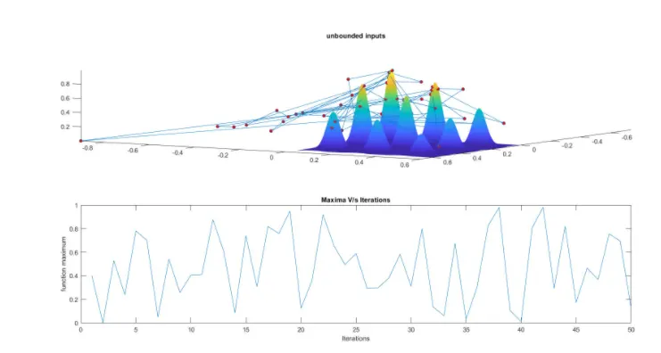
title('Maxima V/S Iterations')

• The first part of the program is the stalgamite function itself & we give the input of [xx,yy] 2D mesh grid to obtain corresponding function output using a for loop.
• These obtained function values are then plotted against xx & yy values using a surface 3D plot. The plot show cases the various local & global maximas.
• Num_cases defines the number of iterations for which we want to run the algorithm.
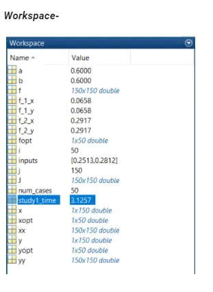
• tic/toc is used to get the time take to run 50 iterations.
• In the next part of the program the genetic algorithm is called and for input arguments the stalgamite function is given as an anonymous function with two design variables ad outputs are the input values of x & y for output optimal function value/global maxima.
• These three variables -xopt, yopt, fopt are plot as a 3D line plot in the same gigure window as the surface plot of stalgamite function Also, another plot is created to show case the maxima value for each of 50 iterations.

Output

Study 2 : To evaluate the algorithms behviour with specifications of bounds but without specification of population size .

clear all
close all
clc

% Creating a search space 
x = linspace(0,0.6,150);
y = linspace(0,0.6,150);

% Creating a 2D mesh 
[xx,yy] = meshgrid(x,y);

% evaluating the stalgamite function
 for i = 1 : length(xx)

for j = 1: length(yy)

a = xx(i,j);
b = yy(i,j);

f_1_x = (sin(5.1*pi*(a)+0.5))^6;
f_2_x = exp(-4*(log(2))*((((a)-0.667)^2/0.64));
f_1_y = (sin(5.1*pi*(b)+0.5))^6;
f_2_y = exp(-4*(log(2))*((((b)-0.0667)^2/0.64));
f(i,j)= -(f_1_x*f_2_x*f_2_y*f_2_y);
end
end

J = -1*f;

num_cases = 50% no.of iterations
%study-2(lower and upper bounds are applied to further restrict the search%space)
tic
for i = 1:num_cases
[inputs,fopt(i)] = ga(@stalagmite,2,[],[],[],[],[0;0],[0.4;0.4]);
fopt(i) = -1*fopt(i);
xopt(i) = inputs(1);
yopt(i) = inputs(2);
end

Study2_time = toc
&plotting
subplot(2,1,1)%creating multiple plots in one figure window
hold on
surfc(xx,yy,J)%stalgamite function surface 3D plot
shading interp %removes grid lines and perfoms shading on the plot 
%plotting the algorithm's behaviour
plot3(xopt,yopt,fopt,'marker','o','markersize',5,'markerfacecolor','r')
title('bouned inputs')
%plotting the optimal function values against the number iterations to %observe the variations in 2D
subplot(2,1,2)
plot(fopt)
xlabel('Iterations')
ylabel('function maximum')
title ('Maxima V/S Iterations')
 

• The first part of the program is the stalagmite function itself and we give the input of [xx,yy] 2D mesh grid to obtain corresponding function output using a for loop.
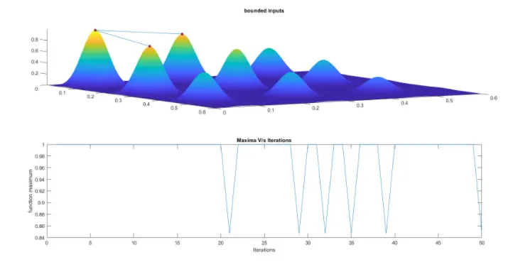
• These obtained function values are then plotted against xx & yy values using a surface 3D plot. The plot show cases the various local& global maximas.
• num_cases defines the number of iterations for which we want to run the algorithm.
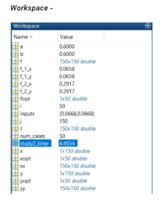
• Tic/toc is used to get the time taken to run 50 iterations.
• In the next part of the program the Genetic algorithm is called & for input arguments the stalagmite function is given an anonymous function with two design variables and this time bounds (upper & lower) are mentioned to restrict the search space & output arguments are the input values of x & y for output optimal function value/global maxima.
• these 3 values -xopt,yopt & fopt are plot as a 3D line plot in the same figure window as the surface plots of stalagmite function . Also, another plot is created to showcase the maxima value for each of 50 iterations.

Output

Study--3 To evaluate the algorithm's behaviour with specification of bounds and population size.

clear all
close all
clc

%Creating a search space

x = linspace(0,0.6,150);
y = linspace(0,0.6,150);

%creating a 2D mesh
[xx,yy] = meshgrid(x,y);

%Evaluating the stalagmite function 
for i = 1:length(xx)
for j = 1:length(yy)

a = xx(i,j);
b = yy(i,j);

f_1_x = (sin(5.1*pi*(a)+0.5))^6;
f_2_x = exp(-4*(log(2))*((((a)-0.0667)^2/0.64));
f_1_y = (sin(5.1*pi*(b)+0.5))^6;
f_2_y = exp(-4*(log(2))*((((a)-0.0667)^2/0.64));
end
end

J = -1.*f;

%Create options (population size) by using optimoptions
options = optimotions('ga');
options = optimotions(options, 'PopulationSize',300);%Increase population size from default 50

num_cases = 50% no.of iterations
%Study-3 (lower & upper bounds and population size is applied %to further restrict the search space & increase the population size from default 50)
tic 
for i = 1:num_cases
[inputs, fopt(i)] = ga(@stalagmite,2,[],[],[],[],[0,0],[0.4,0.4], [],[], options);
fopt(i)= -1*fopt(i);
xopt(i)= inputs(1);
yopt(i) =inputs(2);
end
study2_time = toc 
%plotting
subplot(3,1,1);
hold on 
surfc(xx,yy,J)%stalagmite function surface 3D plot 
shading interp%removes grid lines & performs shading on the plot 
%Plotting the algorithm's behaviour 
plot3(xopt, yopt,fopt, 'marker','o','markersize',5,markerfacecolor','r')
title('bounded inputs')
%plotting the optimal function values against the number iterations to 
%Observe the variations in 2D
subplot(3,1,2)
plot(fopt)
title('Maxima V/S Iterations')
xlabel('Iterations')
ylabel('function maximum')
%Plotting the optimal function values against the number iterations to 
%Observe the variations in 2D with round off values
fopt = round(fopt);
subplot(3,1,3)
plot(fopt)
title('Maxima V/S Iterations (round off values)')
xlabel('Iterations')
ylabel('function maximum')

• The first part of the program is the stalgamite function itself & we give the input [xx,yy] 2D mesh grid to obtain corresponding function output using a for loop.
• These obtained function values are then plotted against xx & yy values using a surface 3D plot. The plot showcases the various local & global maximas.
• Num_cases defines the number of iterations for which we run the algorithm.
• tic/toc is used to get the time taken to run the 50 iterations .
• The default population size chosen by the genetic algorithm is just 50, increasing the value increases the diversity and reduces the average distance between the values. Hence to acheive this options are created by calling the functions optimotions for the algorith 'ga' and the population size is increased to acheive a constant value of maxima.
  • In the next part of the program the Genetic algorithm is called & for input arguments the stalagmite function is given as an annymous function with two design variables and this time bounds(upper & lower) are mentioned to restrict the search space and output arguments are the input values of x & y for output optimal function value/global maxima.
• These three values, -xopt, yopt& fopt are plot as a 3D line plot , in the same figure window as the surface plot of stalgamite function , Also another plot is created to showcase the maxima value for each of 50 iterations.

Output

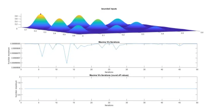
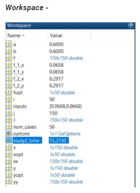
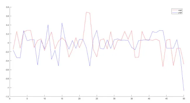
Conclusion : Study 1 shows how algorithm behaves when the bounds are not mentioned , the lack of bounds results in random sampling that is beyond & below the search space that we initially use to evaluate the stalagmite function which leads to random optimal function values for each iteration . The input xopt and yopt for each fopt acheived looks somwthing like this .

Conclusion 2 : With the addtion of upper & lower bounds , the level of randomness in the optimal outputs of the function also reduces which is the result of the defined search space as seen here.

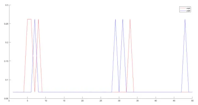
Finally in study 3 the population size specifies how many individuals there are in each generation , with large number population size , the genetic algorithm searches the solution space more thoroughly, thereby reducing the chance that the algorithm returns a local minimum that is not a global minimum, how ever a large population size also causes the algorithm to run more slowly.