Week 4 - Genetic Algorithm
Stalagmite function optimization:
Genetic algorithms:
Genetic Algorithm is a search based optimization technique based on the principles of genetics and natural selection. It is used to find optimal or near optimal solutions to difficult problems.
Optimization: Decision making process which helps find the best results under a set of criteria or constraints.
Genetic algorithm execution:
1.Initialization: Initialization involves the setting up of parameters for the algorithm and creating the scores for the simulation. It can also be defined as a set of chromosomes.
2.Evaluation:The fitness function takes a candidate solution to the problem as input and produces output as how fit or how good the solution is with respect to the problem.
3.Selection and reproduction: Parent selection is the process of selecting parents which help to create best fit soluion.
4.Crossover:The crossover operator is analogous to reproduction and biological crossover. In this more than one parent is selected and one or more off-springs are produced using the genetic material of the parents. Crossover is usually applied in a GA with a high probability
5.Mutation:In simple terms, mutation may be defined as a small random tweak in the chromosome, to get a new solution. It is used to maintain and introduce diversity in the genetic population and is usually applied with a low probability.If the probability is very high, the GA gets reduced to a random search.Mutation is the part of the GA which is related to the “exploration” of the search space. It has been observed that mutation is essential to the convergence of the GA while crossover is not.
Here, the code is written for 3 studies where
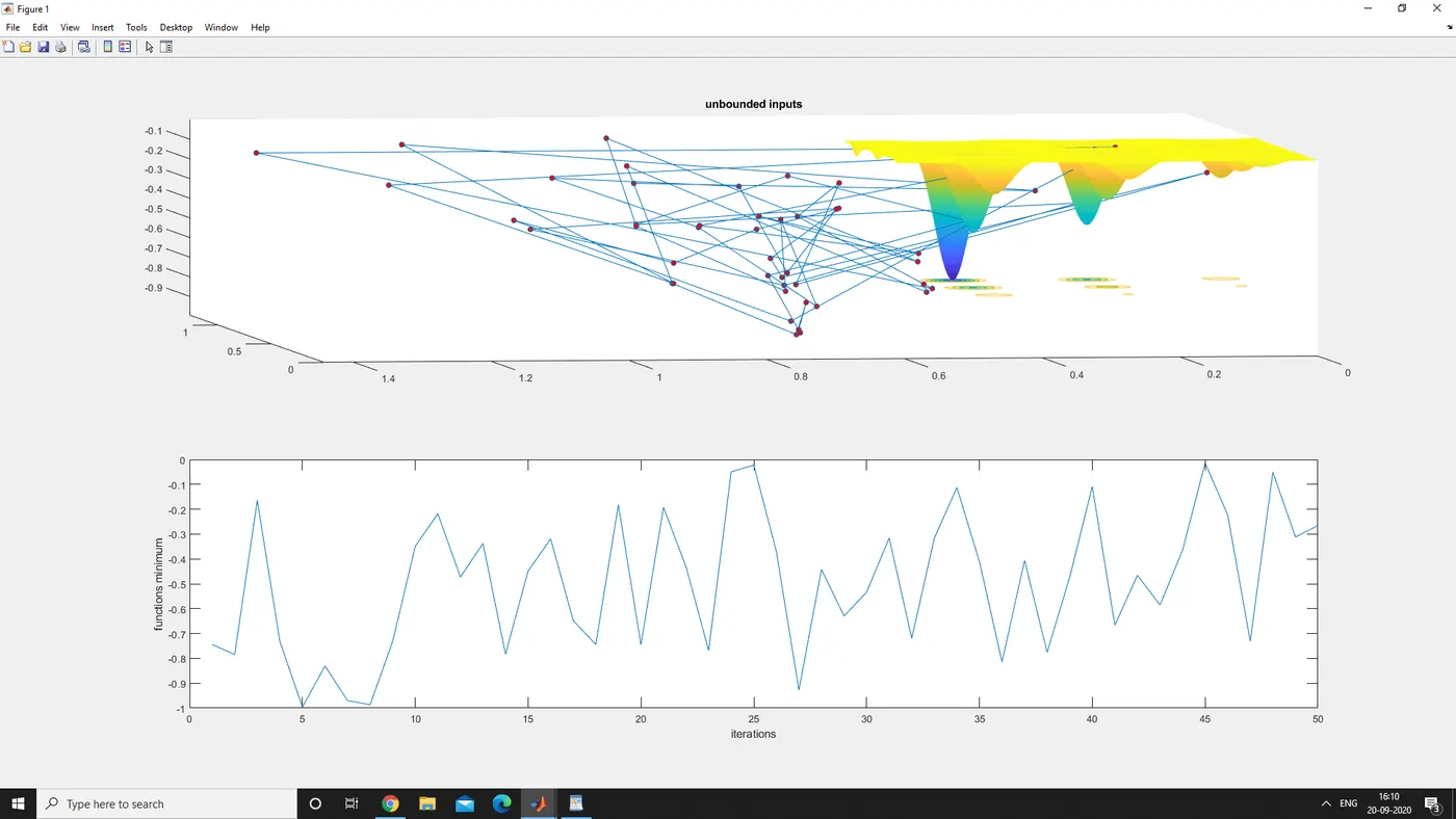
Study1= Finding global maxima.
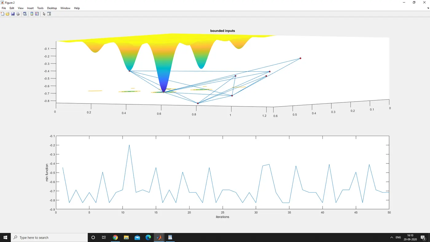
Study2=Statistical behaviour for upper and lower bounds
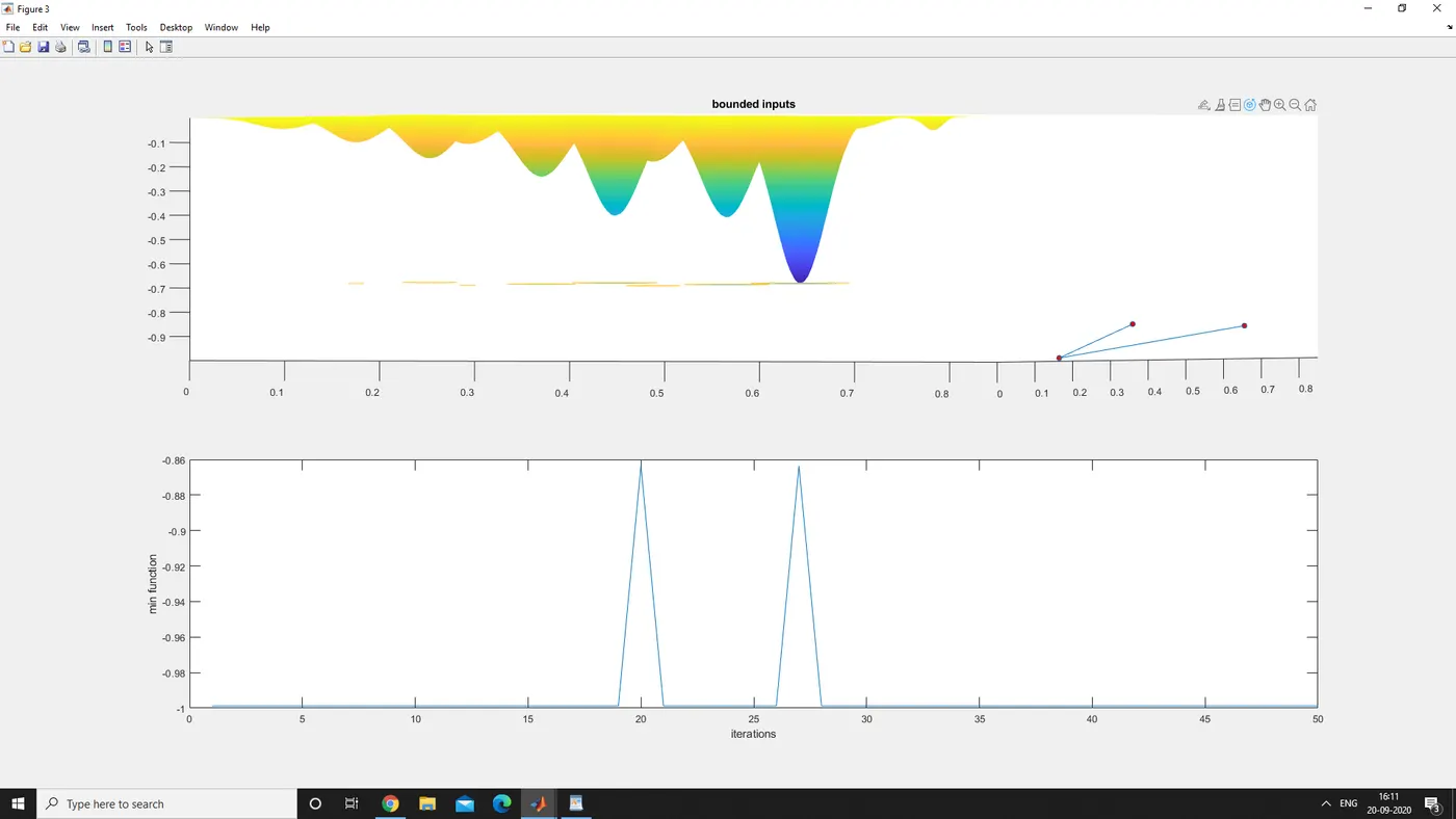
Study3=Statistical behaviour for 200 iterations.
Function code:
function[F]= stalagmite(input_vector)
x=input_vector(1)
y=input_vector(2)
f1_x=(sin(5.1*pi*x+0.5)).^6;
f1_y=(sin(5.1*pi*y+0.5)).^6;
f2_x=exp(-4*log(2)*((x-0.667).^2)/0.64);
f2_y=exp(-4*log(2)*((y-0.667).^2)/0.64);
[F]=-(f1_x.*f1_y.*f2_x.*f2_y);
P=[-F]
end
Stalagmite code:
clear all
close all
clc
%defining our search space
x=linspace(0,0.6,150);
y=linspace(0,0.6,150);
%creating a 2 dimensional mesh
[xx,yy]=meshgrid(x,y);
%Evaluating stalagmite function
for i=1:length(xx)
for j= 1:length(yy)
input_vector(1)=xx(i,j);
input_vector(2)=yy(i,j);
f(i,j)=stalagmite(input_vector);
end
end
surfc(xx,yy,f)
xlabel('x value')
ylabel('y value')
shading interp
[inputs,fval]=ga(@stalagmite,2)
x=linspace(0,0.6,150); %search array
y=linspace(0,0.6,150); %search array
num_case=50 %num case the genetic algorithm is to be run
F=stalagmite(input_vector)
tic
%Study 1-Statistical behaviour
for i=1:num_case
[inputs,fopt(i)]=ga(@stalagmite,2);
xopt(i)=inputs(1);
yopt(i)=inputs(2);
end
study1_time=toc %helps to track time taken to execute program
figure(1)
subplot(2,1,1) %multiple plots inside the same figure window
hold on
surfc(x,y,f)
shading interp
plot3(xopt,yopt,fopt,'marker','o','markersize',5,'markerfacecolor','r') %helps to visualize how algorithm is performing
title('unbounded inputs')
subplot(2,1,2)
plot(fopt)
xlabel('iterations')
ylabel('functions maximum')
tic
%Study2-Statistical behaviour with upper and lower bounds
for i=1:num_case
[inputs,fopt(i)]=ga(@stalagmite,2,[],[],[],[],[0:0],[0.6:0.6]);
xopt(i)=inputs(1);
yopt(i)=inputs(2);
end
study2_time=toc
figure(2)
subplot(2,1,1)
hold on
surfc(x,y,f)
shading interp
plot3(xopt,yopt,fopt,'marker','o','markersize',5,'markerfacecolor','r')
title('bounded inputs')
subplot(2,1,2)
plot(fopt)
xlabel('iterations')
ylabel('min function')
%Study3-Increasing GA iterations
options=optimoptions('ga');
options=optimoptions(options,'populationsize',200);
tic
for i =1:num_case
[inputs,fopt(i)]=ga(@stalagmite,2,[],[],[],[],[0;0],[1;1],[],[],options); %minimizes default optimization parameters replaced by values in options
xopt(i)=inputs(1);
yopt(i)=inputs(2);
end
study3_time=toc
figure(3);
subplot(2,1,1)
hold on
surfc(x,y,f)
subplot(2,1,1)
hold on
surfc(x,y,f)
shading interp
plot3(xopt,yopt,fopt,'marker','o','markersize',5,'markerfacecolor','r')
title('bounded inputs')
subplot(2,1,2)
plot(fopt)
xlabel('iterations')
ylabel('min function')
Graphs:
1.Study 1
2.Study 2
3. Study 3:
Code Explained:
We start off by creating an array of x and y values. The stalagmite code is written as a calling function.To get the best fit iteration times are mentioned using num_case to obtain satisfactory end values. For loops are used to run codes for Study 1&2 as writing full length code would become tedious.Subplots are used for all the three studies to provide plots for multiple values.Plot helps us to visualize algorithm performance.Study 1 provides us the global maxima and negative sign is given to final value of stalagmite as stalagmite usually provides us with the minimum value. For study 2, Upper and Lower bounds are provided. Study 3 has increased iterations to provide us with max value. Time taken to execute the code is found by using tic-toc command.
Run time:
Study1=42.3997s
Study2=28.1900s
Study3=104.7840s
Errors faced:
1. Calling stalagmite function proved to be an issue due to differences in calling names. Issue was fixed when the correct name was used.
2. Population Size issue was corrected when it was rewritten as populationsize.
3.Minor issues with study 3 plot which was due to typing error(, was missing).
Advantages of Genetic Algorithms:
1. Efficient compared to other methods.
2. Optimizes continuous and discrete functions for multi objective problems.
3. Provides the best solution and not just one solution.
4.Gets an answer which becomes better over time.
5.Useful when search space is large and various parameters are involved.
Limitations:
1. Fitness value is calculated repeatedly which might be computationally expensive for some problems.
2. Being stochastic, there are no guarantees on the optimality or the quality of the solution.
3. Genetic algorithm may not converge the optimal solution.
Uses:
Optimization,economics,neural networks,image processing,vehicle routing, scheduling applications,machine learning,design problems,dna analysis,operations research.
Resources:
2.https://www.tutorialspoint.com/genetic_algorithms/genetic_algorithms_introduction.htm