Week 4 - Genetic Algorithm

GENETIC ALGORITHM:

The genetic algorithm is a method for solving both constrained and unconstrained optimization problems that are based on natural selection, the process that drives biological evolution. The genetic algorithm repeatedly modifies a population of individual solutions. At each step, the genetic algorithm selects individuals at random from the current population to be parents and uses them to produce the children for the next generation. over successive generations, the population evolves toward an optimal solution. You can apply the genetic algorithm to solve a variety of optimization problems that are not well suited for standard optimization algorithms, including problems in which the objective function is discontinuous, nondifferentiable, stochastic, or highly non-linear. The genetic algorithm can address problems of mixed-integer programming, where some components are restricted to be integer-valued.

The genetic algorithm uses three main types of rules at each step to create the next generation from the current population:

Selection rules: select the individuals, called parents that contribute to the population at the next generation.

Crossover rules: combine two parents to form children for the next generation.

Mutation rules: apply random changes to individual parents to form the children.

Genetic algorithms are primarily used in optimization problems of various kinds, but they are frequently used in other application areas as well.

The areas in which Genetic algorithms are frequently used are listed below.

Optimization:

Genetic algorithms are most commonly used in optimization problems wherein we have to maximize or minimize a given objective function value under a given set of constraints.

Economics:

GAs are used to characterize various economic models like the cobweb model, game theory equilibrium resolution, asset pricing, etc.

Neutral Networks:

GAs are used to train neural networks, particularly recurrent neural networks.

Image processing:

GAs are used for various digital image processing(DIP) tasks as well as dense pixel matching.

The above are some of the areas where the genetic algorithm is extensively used for optimization.

FITNESS FUNCTION:

The fitness function takes the solution as input and produces the suitability of the solution as the output. This evaluates how close the solution is to the optimal solution of the desired problem.

The syntax for GA in Matlab:

x=ga(fun,nvars,A,B,Aeq,Beq,lb,ub,nonlcon,Intcon,options)

This syntax is explained as follows:

'x' is the variable to store the output of the genetic algorithm.

'fun' is the function handle to call the function.

'A' and 'B' are used to represent the linear inequalities of the function, if the linear inequalities do not exist, they can be set as empty[].

Aeq and Beq are used to represent the equality constraints. similarly, if the linear equalities do not exist, they can be set as empty[].

'lb' and 'ub' are used to specify the upper and the lower bounds of the variables of the function.

'nonlcon' represents the non-linear constraints.

Intcon represents the integer constraint, such that the value of the function is an integer.

'options' used to provide the value of the default parameters used named parameters, if it is required to replace the default parameters. This is done by using the 'optimoptions'

Stalagmite Function:

A Stalagmite is an upward-growing mound of mineral deposits that have precipitated from water dripping onto the floor of a cave. Most stalagmites have rounded or flattened tips.

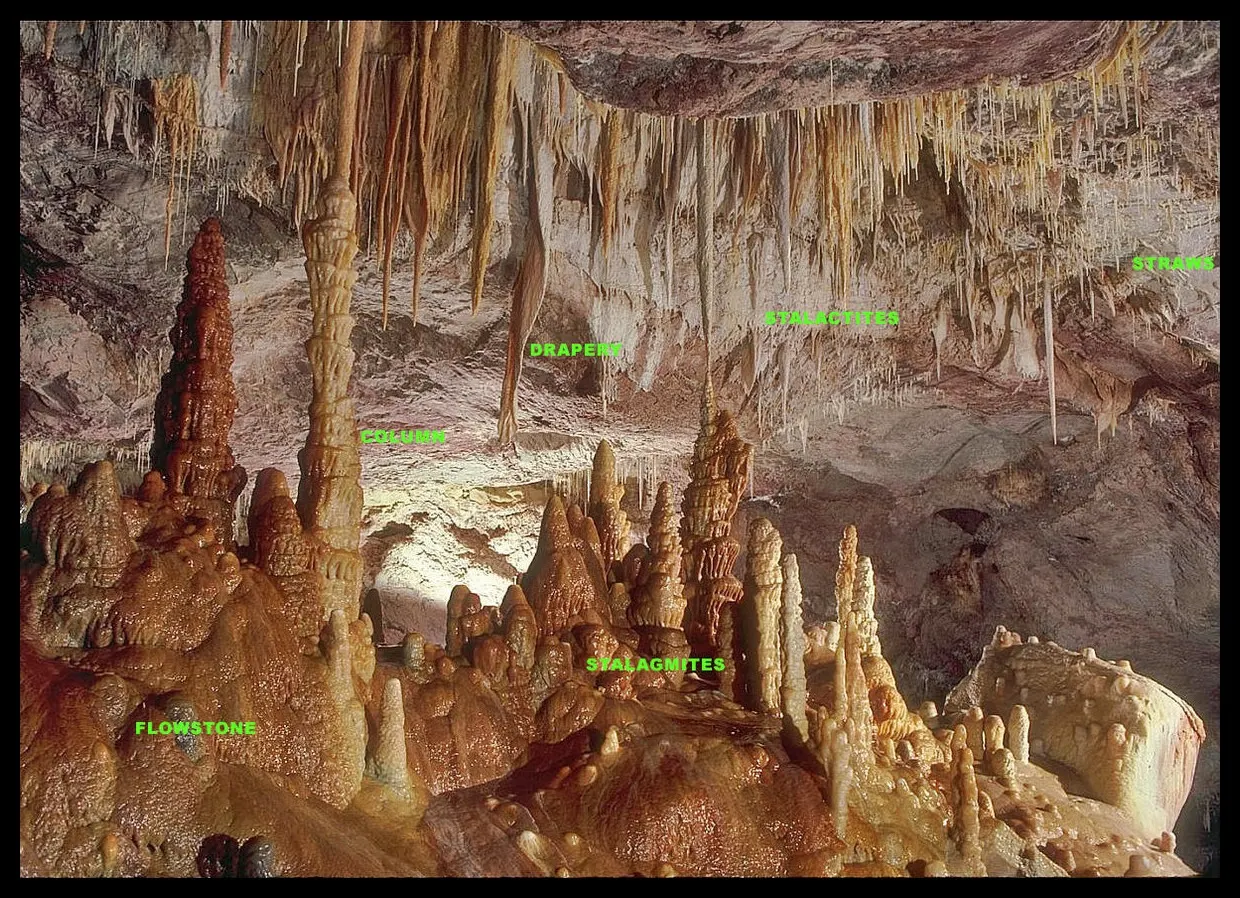
The following function will look like this feature hence it is called the stalagmite function.

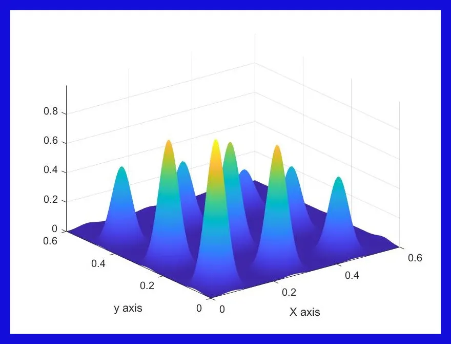
The following is the given stalagmite function for which we need to find the global maxima.

`f(x,y)=f1x*f2x*f1y*f2y`

where,

`f1x=[sin(5.1pix+0.5)]^6`

`f1y=[sin(5.1piy+0.5)]^6`

`f2x=exp[-4ln(2)*(x-0.0667)^2/0.64]`

`f2y=exp[-4ln(2)*(y-0.0667)^2/0.64]``

Function program:

function [f]=stalagmite(input_vector)

a=input_vector(1);
b=input_vector(2);

f1_x=[sin((5.1*pi*a)+0.5)].^6;
f1_y=[sin((5.1*pi*b)+0.5)].^6;
f2_x=exp(-4*log(2)*(((a-0.0667)^2)/(0.64)));
f2_y=exp(-4*log(2)*(((b-0.0667)^2)/(0.64)));

f=-(f1_x*f1_y*f2_x*f2_y);

end

• The negative command is used in the program in order to invert the plot as the ga command finds only the minimum point.

Main Program:

clear all
close all
clc

x=linspace(0,0.6,150);
y=linspace(0,0.6,150);

[xx yy]=meshgrid(x,y);

for i=1:length(xx)    
    for j=1:length(yy)
        input_vector(1)=xx(i,j);
        input_vector(2)=yy(i,j);
        f(i,j)=stalagmite(input_vector);
    end
end


surfc(xx,yy,f)
shading interp

[inputs,fval]=ga(@stalagmite,2)

xlabel('X axis')
ylabel('y axis')

• Clear all, close all and clc represents it deletes all temporary memory, closes all plots, and clears the command window.
• We assume x and y values using the linspace command. The uses of linspace command are that if we set lower and upper limits and the number of values we need it takes random values.
• In the next step, the mesh grid command is used in order to form an array of row and column values and it is stored in xx and yy variables.
• Then, for loop command is used. It repeats the function for the length of xx and yy.
• Then in the next step, we call the stalagmite function as stalagmite(input_vector).
• In the next step, surfc command is used in order to get a plot as a surface.
• Then, shading interp command is used in order to remove the grid-like structure in the plot, and color filling is done.you can refer it in the following figure.
• In the next step, the ga command is used. In the ga command, we call the stalagmite function and we need to enter the number of variables. In our problem, we have two variables x and y so we enter it as 2.
• Then in the next step x label and y label is used in order to get a clear picture of our plot.

Study-1 Statistical Behavior:

%STUDY-1 Statistical Behavior
num_cases=50

tic
for i=1:num_cases
    [inputs1,fopt1(i)]=ga(@stalagmite,2);
    xopt1(i)=inputs1(1);
    yopt1(i)=inputs1(2);
end
study1_time=toc;
mean1=-(mean(fopt1))

figure(1)
subplot(2,1,1)
hold on
surfc(x,y,-f)
shading interp
plot3(xopt1,yopt1,-fopt1,'marker','o','markersize',5,'markerfacecolor','r');
title('Unbounded inputs')
xlabel('X-Axis')
ylabel('Y-Axis')
subplot(2,1,2)
plot(fopt1)
xlabel('Iterations')
ylabel('Function minimum')

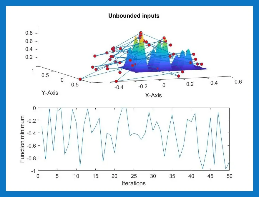
• In this study, we introduce the number of cases that ga needs to perform, and based on the mean value we need to calculate our global maximum value.
• We define it as num_cases=50 in this program. The 50 indicates that 50 times the ga need to repeat and it calculates the value.
• The tic command is used in order to find out the time taken for the program to complete.
• For loop command is used and the length of it set as the number of cases.
• Then ga command is used as before by calling the function and the number of variables in the program.
• The calculated x and y values are stored in xopt(i) and yopt(i).
• subplot command is used in order to get n number of plots in the same single figure plot.
• In the first plot, we plot the x,y, and f as a surface like structure by using the surf command.
• The negative sign is used in the function (f) while plotting since we invert initially and we need to revert it back to its original structure.
• Then we plot calculated maximum value as a dot-like structure by using the marker opting and marker size.
• In the next step title for the is mentioned using the title command.
• Then subplot command is used in order to plot in the same figure window.
• In this plot, we plot the values and the number of iterations, and the x label and y label is mentioned.
• In this study, we get a random value and we didn't get an exact global maximum value and the search space of ga is also not within our search space.
• Thus it indicates we need to have a better study method through which we get our exact global maximum value within our search space.

Study-2 Statistical Behavior with upper and lower bound limits:

%study-2 statistical behavior with upper and lower bounds

tic
for i=1:num_cases
    [inputs2,fopt2(i)]=ga(@stalagmite,2,[],[],[],[],[0,0],[1,1]);
    xopt2(i)=inputs2(1);
    yopt2(i)=inputs2(2);
end
study2_time=toc;
mean2=-(mean(fopt2))


figure(2)
subplot(2,1,1)
hold on
surfc(x,y,-f)
shading interp
plot3(xopt2,yopt2,-fopt2,'marker','o','markersize',5,'markerfacecolor','r');
title('Bounded inputs')
xlabel('X-Axis')
ylabel('Y-Axis')
subplot(2,1,2)
plot(fopt2)
xlabel('Iterations')
ylabel('Function minimum')

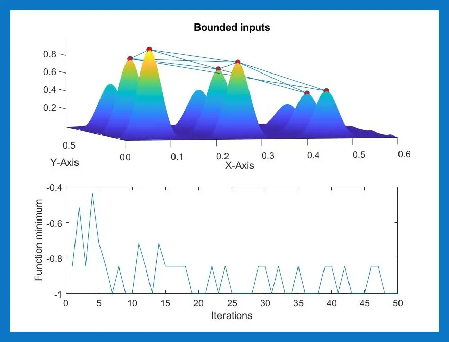
• From the previous study, we inferred that the search space of the ga is not within our search space so to overcome this error we use the bounded script method.
• As the name suggests, in this study we will enter the boundary and within that boundary, only the ga will perform.
• All the commands used in this study are also the same as used in the previous study except the ga syntax.
• In this study as mentioned above the limit criteria, Initially, we call the stalagmite function and the number of variables mentioned as done earlier, and we enter the lower and upper boundary limit values.
• In our program, the lower boundary limit is set as 0,0 and the upper boundary limit is set as 1,1.
• After this, we plot the same way as before and we get our plot.
• Based on the output we inferred that even though this study is better than our previous study but still we didn't an exact single global maximum value.

Study-3 Increasing GA Iterations:

%study-3 Increasing GA iterations

options=optimoptions('ga');
options=optimoptions(options,'populationsize',400);


tic
for i=1:num_cases
    [inputs3,fopt3(i)]=ga(@stalagmite,2,[],[],[],[],[0,0],[1,1],[],[],options);
    xopt3(i)=inputs3(1);
    yopt3(i)=inputs3(2);
end
study3_time=toc;
mean3=-(mean(fopt3))

figure(3)
subplot(2,1,1)
hold on
surfc(x,y,-f)
shading interp
plot3(xopt3,yopt3,-fopt3,'marker','o','markersize',5,'markerfacecolor','r');
title('Bounded inputs with modified population size')
xlabel('X-Axis')
ylabel('Y-Axis')
subplot(2,1,2)
plot(fopt3)
xlabel('Iterations')
ylabel('Function minimum')

• All the commands used in this study are also the same as used in the previous study except the ga syntax.
• In the previous study, we set the lower and upper boundary limits but we didn't set the initial population size for the ga to perform.
• Thus in this optimization technique, we will try to set the initial population size that ga needs to perform within our boundary limits.
• Thus to set the initial population size we use the optimoptions command and in that we mention the options, population size.
• After this, we plot the same way as before and we get our plot.
• The population value is randomly increased up to which a single exact global maximum value is found out.
• By increasing like this we get a single exact point at the population size of 300.so we stop our program at this point.

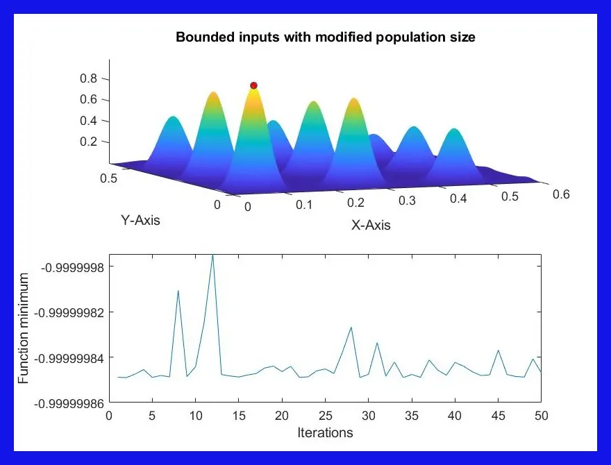
RESULTS:

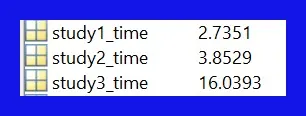
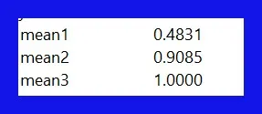
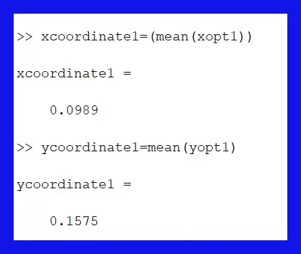
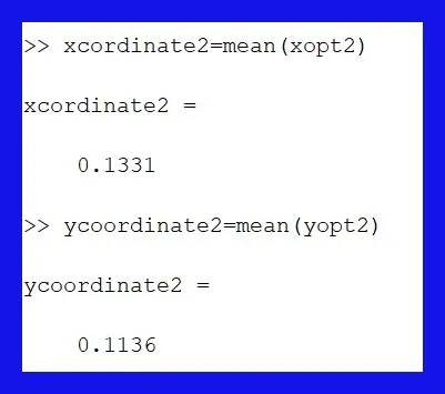
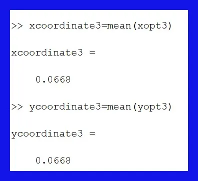
The time taken for the study, Global Maximum value and the coordinate values of x and y are found out for each study and the results are shown below:

CONCLUSION:

• Understand how optimization technique is used with the ga command.
• Understand the function of ga and it uses.
• Understand how to improve our program step by step through different studies.