Week 4 - Genetic Algorithm

Genetic Algorithm

INTRODUCTION:

At first, the coding to be used must be defined. Then using a random process, an initial population of strings is created. Next, a set of operators is used to take this initial population to generate successive populations, which hopefully improve with time. The main operators of the genetic algorithms are reproduction, crossover, and mutation.

Reproduction is a process based on the objective function (fitness function) of each string. This objective function identifies how “good” a string is. Thus, strings with higher fitness value have bigger probability of contributing offsprings to the next generation.

Crossover is a process in which members of the last population are mated at random in the mating pool. So, a pair of offsprings is generated, combining elements from two parents (members), which hopefully have improved fitness values. Mutation is the occasional (with small probability) random alteration of the value of a string position. In fact, mutation is a process of random walk through the coded parameter space. Its purpose is to ensure that important information contained within strings may not be lost prematurely.

The implementation of GAs to the problem of optimization of operation and site-scale energy use in production plants is envisaged to be carried along the following lines.

First, using the pinch design method, the problem requirements and constraints will be defined. Next, the region of the pinch will be identified, and the essential matches will be made. Then, the problem will be coded by generating the appropriate strings. These strings will contain the general features and the parameters, which affect the problem. Each string will represent a possible network configuration. For each one of the strings, the objective function will be calculated, that is, the value of energy and utility usage and the number of units need to be used in the represented network configuration, that is, the total capital and operating cost. Initially, a starting population of strings will be created using a random procedure. The three main operators of the genetic algorithms will be performed to improve the value of the objective function, namely, to create network configurations with minimal total capital and operating cost. To the final population of strings/possible networks, advanced techniques will be applied for further improvement.

Genetic algorithm is a kind of stochastic algorithm based on the theory of probability. In application this method to a stagewise superstructure model, the search process is determined by stochastic strategy. The global optimal solution for the synthesis of heat exchanger networks can be obtained at certain probability. The search process begins with a set of initial stochastic solutions, which is called “population.” Each solution is called “chromosome,” the chromosome is composed of “gene,” and the “gene” stands for the optimal variables of heat exchanger networks, for example, the mass flowrates of cold streams and hot streams.

MATLAB CODE:

clear all 
close all
clc

%input values
x=linspace(0,0.6,150);
y=linspace(0,0.6,150);

[xx yy]=meshgrid(x,y);
num_case=100;

for i=1:length(xx)
    for k=1 : length(yy)
        input_vector(1)=xx(i,k);
        input_vector(2)=yy(i,k);
        f(i,k)=stalagmite(input_vector);
    end
end

%Study (without bounds)
tic
for i=1:num_case
    [inputs,fopt(i)]=ga(@stalagmite,2);
    xopt(i)=inputs(1);
    yopt(i)=inputs(2);
end

Study_time_1=toc

figure(1)
subplot(2,1,1);
hold on
surfc(xx,yy,f);
shading interp;
ylabel('y data');
xlabel('x data');
plot3(xopt,yopt,fopt,'marker','o','markersize',10,'markerfacecolor','b');
title('Unbounded inputs');
subplot(2,1,2);
plot(fopt);
xlabel('Iterations');
ylabel('maximum value of function');

%Study 2 (with upper and lower bounds)
tic
for i=1:num_case
    [inputs,fobt(i)]=ga(@stalagmite,2,[],[],[],[],[0:0],[1:1]);
    xopt(i)=inputs(1);
    yopt(i)=inputs(2);
end

study_time_2=toc

figure(2)
subplot(2,1,1);
hold on
surfc(xx,yy,f);
shading interp;
ylabel('y data');
xlabel('x data');
plot3(xopt,yopt,fopt,'marker','o','markersize',10,'markerfacecolor','b');
title('bounded inputs');
subplot(2,1,2);
plot(fopt);
xlabel('interations');
ylabel('Maximum value of function');


%Study 3 
options=optimoptions('ga');
options=optimoptions(options,'populationsize',200);
tic
for i=1:num_case
    [inputs,fopt(i)]=ga(@stalagmite,2,[],[],[],[],[0:0],[1:1],[],[],options);
    xopt(i)=inputs(1);
    yopt(i)=inputs(2);
end

study_time_3=toc

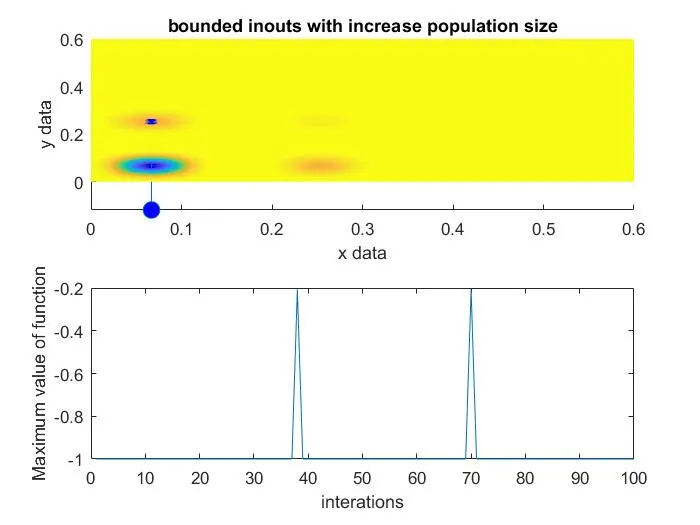
figure(3)
subplot(2,1,1);
hold on
surfc(xx,yy,f);
shading interp;
ylabel('y data');
xlabel('x data');
plot3(xopt,yopt,fopt,'marker','o','markersize',10,'markerfacecolor','b');
title('bounded inouts with increase population size');
subplot(2,1,2);
plot(fopt);
xlabel('interations');
ylabel('Maximum value of function');

max_value=fopt

FUNC_CODE:

function [f] = stalagmite(input_vector)
x = input_vector(1);
y = input_vector(2);
f_1x=(sin(5.1*pi*x+0.5))^6;
f_1y=(sin(5.1*pi*y+0.5))^6;
f_2x=exp(-4*log(2)*((x-0.0667)^2/0.064));
f_2y=exp(-4*log(2)*((y-0.0667)^2/0.064));
f=-(f_1x*f_1y*f_2x*f_2y);
end

PROCEDURE:

• Initially stalagmite code has been written.
• A nagative sign is used for function to obtainfrom maximum and minimum.
• A Nested for-loop is utilize to iterate each of elements.
• Then the plot command has been written.
• The main progaram code saved and named stalagmite_main.m.
• Then the function code was saved stalagmite.m
• The function which is used to call the function code with a help of call function option.
• In this task there are three types of input plots are given.
• Finally the progaram has runned ,than the plots are drawn.

FINAL RESULT:

FIG_NO: 01

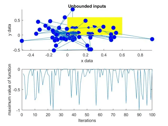
FIG_NO: 02

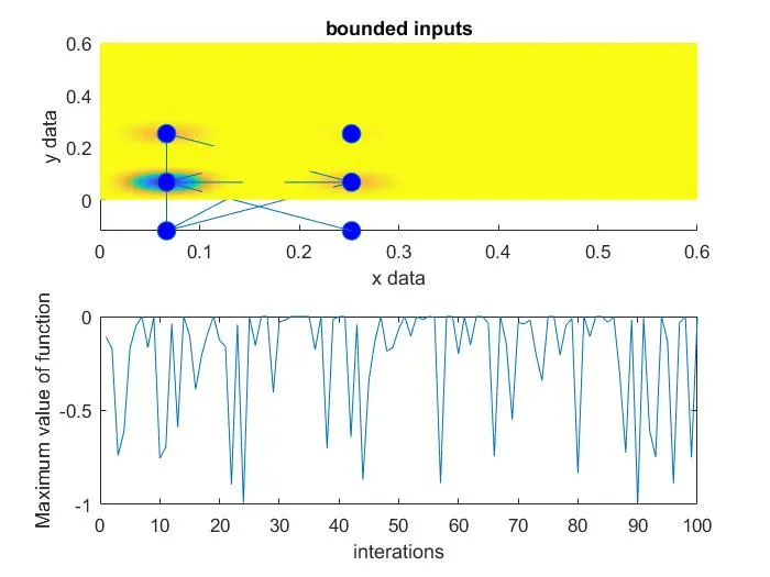
FIG_NO: 03