Week 4 - Genetic Algorithm

Aim - Write a code in MATLAB to optimise the stalagmite function and find the Global Maxima .

Objective –

1. Write a Genetic Algorithm for optimization .
2. Find the Global maxima for function .

Introduction

Optimization –

It is the selection of the best element from a set of known elements .This is used in many engineering and other areas where a best result is required without spending much time in trial and error method .

Genetic Algorithm (G A) -

It is a search based optimization technique ,based on the idea of natural selection . This algorithm reflects the process of natural selection where fittest individuals are selected for reproduction in order to produce offspring of the next generation .

In MATLAB the Ga is an in-built function which is a method for solving both the constrained and unconstrained optimization problems .It mainly uses three types of rules at each step ,which are : -

Selection rules – selects the individual ,called parent that contribute to next population .

Crossover – To combine two parents to form one .

Mutation rule – Apply random changes to produce the children .

Syntax of G A –

[input , fval] = ga(f, n_var , A, B, Aeq , Beq, lb, ub, non_lcon, options )

Where ,

f - Fitness function or also called the Objective Function .

n_var – The number of design or optimization variables

A , B– linear in -equalities

Aeq , Beq - linear equalities

Lb ,ub - Lower bound and upper bound

Non_lcon - non linear constraint

Options - create options using “optimoptions” .

Stalagmite –

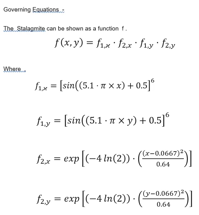
It is type of rock formation that rises at the caves due to accumulation of materials from ceiling drippings . It can be plotted using a function f .Which is defined below .

Code -

clc
clear all
close all

%defining the workspace .....
x = linspace(0,0.6,150) ;
y = linspace(0,0.6,150) ;
%creating 2 - D array ......
[xx,yy] = meshgrid(x,y);

% evaluating stalgamite function ....
for i = 1 : length(xx) 
    for j = 1 : length(yy) 
        input_vector(1) =  xx(i,j) ;
        input_vector(2) =  yy(i,j) ;
        f(i,j) = stalgamite_function(input_vector) ;
        
    end
end


%% study - 1 ...unbounded  optimization ....

num_cas = 40 ;
tic  % used for the timer /..
for n = 1 : num_cas 
    [ inputs , f1(n) ]  = ga(@stalgamite_function,2);
    x1(n) = inputs (1) ;
    y1(n) = inputs (2) ;
    
end

study_time_1 = toc; 

% plot......
figure (1) 

grid on ;
subplot(2,1,1)
surf(xx , yy , -f ) ;
shading interp  ;
colorbar ;
title('unbounded optimization ') ;
hold on ;
plot3(x1 , y1 , -f1 ,'marker', 'o','Markersize',4,'MarkerFaceColor','r' );
xlabel('X - axis ') ;
ylabel('Y- axis ') ;

subplot(2,1,2)
plot(-f1) ;
xlabel('no. of iterations '); 
ylabel('Max value of function ') ;



%% study - 2 ...bounded  optimization ....


tic 
for n = 1 : num_cas 
    [inputs2 , f2(n) ]  = ga(@stalgamite_function,2,[],[],[],[],[0;0],[1;1]);
    x2(n) = inputs2(1); 
    y2(n) = inputs2(2) ;
    
end

study_time_2 = toc; 

% plot......

figure  (2) 

grid on ;
subplot(2,1,1)
surf(xx , yy , -f ) ;
shading interp  ;
colorbar ;
title('bounded optimization ') ;
hold on ;

plot3(x2 , y2 , -f2 , 'o','Markersize',4,'MarkerFaceColor','r' );
xlabel('X - axis ') ;
ylabel('Y- axis ') ;

subplot(2,1,2)
plot(-f2) ;
xlabel('no. of iterations '); 
ylabel('Max value of function ') ;



%% study - 3 ...bounded  optimization  with increased population ....
options = optimoptions('ga') ;
options = optimoptions('ga','populationSize',180) ;

tic 
for n = 1 : num_cas 
    [ inputs3 , f3(n) ]  = ga(@stalgamite_function,2,[],[],[],[],[0;0],[0.8;0.8],[],[],options);
    x3(n) = inputs3(1); 
    y3(n) = inputs3(2) ;
    
end

study_time_3 = toc; 
% plot......

figure  (3) 

grid on ;
subplot(2,1,1)
surf(xx , yy , -f ) ;
shading interp  ;
colorbar ;
title('bounded optimization with increased population  ') ;
hold on ;

plot3(x3 , y3 , -f3 , 'o','Markersize',4,'MarkerFaceColor','r' );
xlabel('X - axis ') ;
ylabel('Y- axis ') ;

subplot(2,1,2)
plot(-f3) ;
xlabel('no. of iterations '); 
ylabel('Max value of function ') ;

Stalagmite_function –

function f  = stalgamite_function(input )

a = input(1) ;
b =  input(2) ;

p = (sin((5.1*pi*a)+0.5))^6 ;

q = (sin((5.1*pi*b)+0.5))^6 ;

r = exp(-4*log(2)*((a - 0.0667)^2/0.64));

s = exp(-4*log(2)*((b - 0.0667)^2/0.64));

f = -(p*q*r*s) ;  % it is used to find the maxima of the function .....



end

Explanation -

1. The first three lines of the code are used to refresh the workspace .
2. The values of x and y is defined which shows the workspace .
3. It is then converted in to two d array using meshgrid command .
4. now using a for loop the the optimum value for the function is calculated by calling the objective function .
5. Now a study 1 is conducted , which unbounded optimization .
6. Tic command is used as atimer .
7. The number of iterations is specified using the variable "num_cas ".
8. now a for loop is used till the iteration .The bulit- in ga function is used to determine the maximum value ,at x and y .
9. This value is then plotted .A surf plot is plotted with the optimum values which the ga function predicted is ploted together.Another plot where maimum value and number of iterations is plotted .
10. After study 1, it is seen that the ga function takes values which is out of the workspace.Now to correct this an bounded optimization which is the study 2 is conducted .
11. The only change in the code is the number of inputs to the ga function . The lower bound and upper bound is now provided to specifiy the boundaries .

12. % The linear inequalities and linear equalities are not provided thus an empty array is used ..
    % The lower and upper bound is specified ...
    for n = 1 : num_cas 
        [inputs2 , f2(n) ]  = ga(@stalgamite_function,2,[],[],[],[],[0;0],[1;1]);
        x2(n) = inputs2(1); 
        y2(n) = inputs2(2) ;
        
    end

13. After this the values that are obtained are plotted simillarly as the study 1 .
14. Now study 3 is conducted where The population size is increased to 180 .

15. options = optimoptions('ga') ;
    options = optimoptions('ga','populationSize',180) ;
    
    tic 
    for n = 1 : num_cas 
        [ inputs3 , f3(n) ]  = ga(@stalgamite_function,2,[],[],[],[],[0;0],[0.8;0.8],[], 
                                                                                 [],options);
    
        x3(n) = inputs3(1); 
        y3(n) = inputs3(2) ;
        
    end

16. After the values are plotted the graph is now plotted simmar to the above studies .

Result -

STUDY 1 -

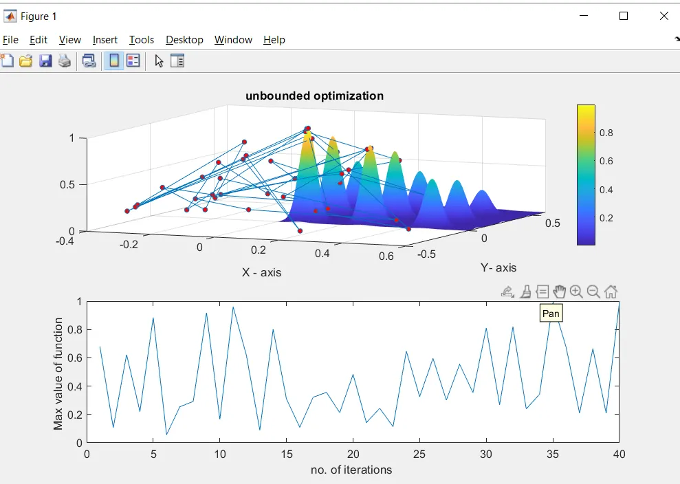
From the The above first plot it can be seen that the ga function predicts the maximum value but out of the workspace. The boundary is not specified for it . Also For a certain amount of iterations the maximum value obtained is not constant . Thus it can be said that the plot obtained is not correct .

STUDY 2 -

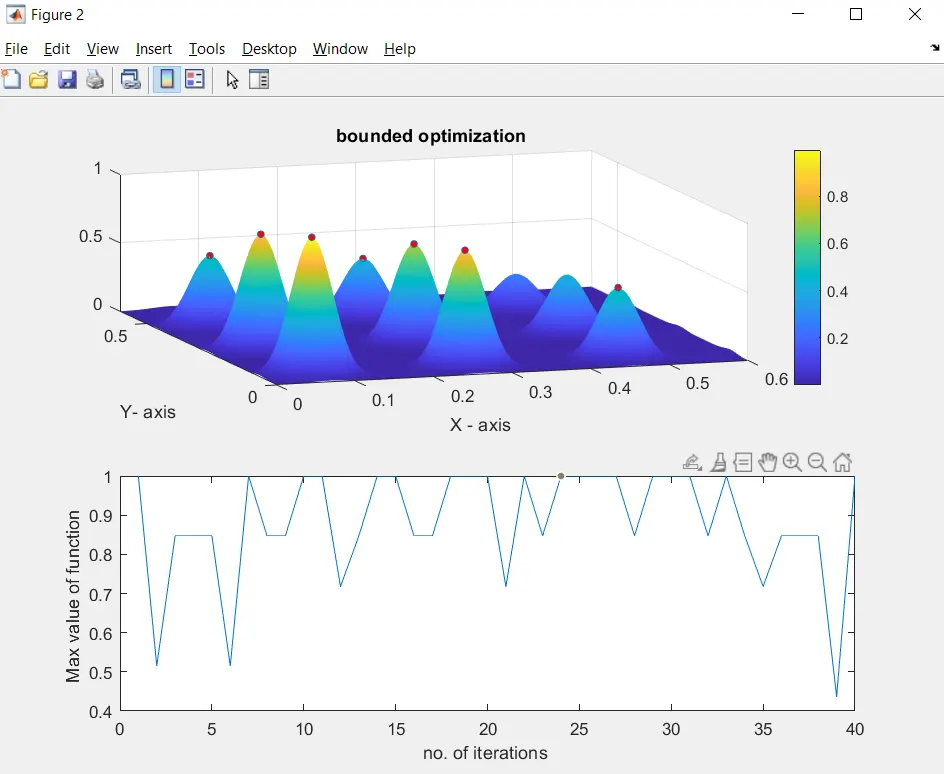
From the above plo0t it can be seen that the maximum value obtained is now within the boundary limits .But still the maximum value over a number of iterations are not constant .This can be improved by increasing the number of population size .

STUDY 3 -

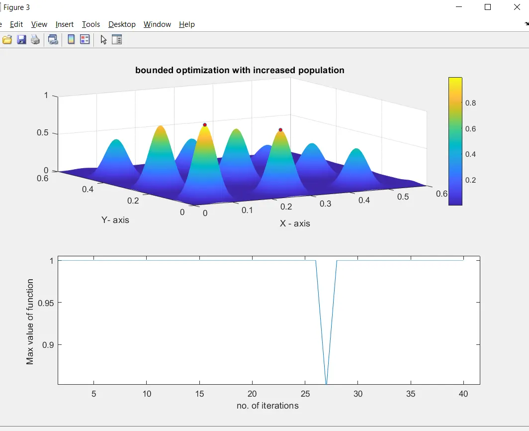
From The above plot it can be seen that the maximum value now exits between the two peeks .Also in the second plot the maximum value is constant and only at a single value the maximum value becomes 0.86 .

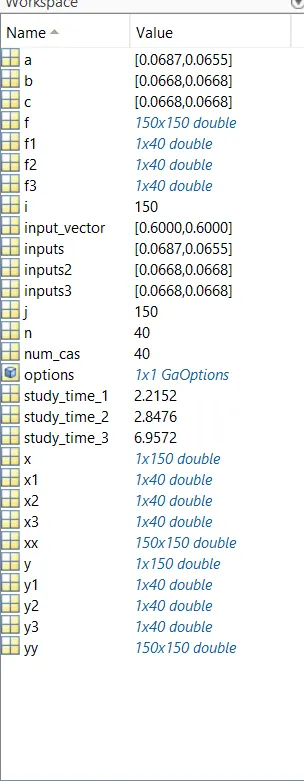
The only error obtained was getting minimum value everytime . This was solved by multiplying the objective function value by a (-1) .

f = -(p*q*r*s) ;  % it is used to find the maxima of the function .....

Conclusion -

When the population size is increased more number of individuals are taken from inside the bounded reigion by the ga ()function .

Thus the objective of the programe is completed .

References -

https://in.mathworks.com/help/gads/ga.html