Week 4 - Genetic Algorithm

Aim:

To write a MATLAB code to optimize the stalagmite function and find the global maxima of the function.

Algorithm:

1. A coordinate system is first initialized to fix the working space of the function using the genetic algorithm.
2. The number of iterations is decided and initialized within the input initialization part of the program
3. The stalagmite function is defined in a separate file as per its mathematical definition.
4. The stalagmite function is called in the main function and the mesh grid generated in the main program is initialized for the stalagmite function using the loop function of the MatLab.
5. Next is the initialization of the three cases as per the use of the genetic algorithm.
6. The three cases will be according to the syntax of the genetic algorithm. These cases are the unbounded case, bounded case, and lastly optimized function bounded case.
7. Each case will have plot commands generating the various contours for the visual representation of the global maxima that has to be found out using this program.

MATLAB code:

• Main code

clear all
close all
clc

%inputs
x=linspace(0,0.6,150);
y=linspace(0,0.6,150);
n=50; % total number of cases

%prepartion of the stalagmite function

for i= 1:length(x)
for j= 1:length(y)
input_vector(1)=x(i);
input_vector(2)=y(j);

f(i,j)= stalagmite(input_vector);
end
end

% case 1 statistacial behavior
tic
 for k=1:n
 [ip1 fopt1(k)]=ga(@stalagmite,2)
 xopt1(k) = ip1(1)
 yopt1(k) = ip1(2)
 end

study1_time=toc
 figure(1)
 subplot(2,1,1)
 hold on
 surfc(x,y,-f)
 shading interp


 plot3(xopt1,yopt1,-fopt1,'marker','o','markerfacecolor','r')
 
 xlabel ('iterations')
 ylabel ('function maxima')
 title ('statistical behavior')


figure (2)
plot(-fopt1)
xlabel('iterations')
ylabel('fopt1')
title('unbounded plot')



%case 2 statistical behavior with upper and lower bounds
tic
for k=1:n

[ip2 fopt2(k)]= ga(@stalagmite,2,[],[],[],[],[0;0],[1;1])
xopt2(k)= ip2(1)
yopt2(k)=ip2(2)

end
study2_time=toc
figure(3)
subplot(2,1,1)
hold on
surfc(x,y,-f)
shading interp

plot3(xopt2,yopt2, -fopt2,'marker','o','markerfacecolor','r')
xlabel('x values')
ylabel('y values')
title('bounded plot')

figure(4)
plot(-fopt2)
xlabel('iterations')
ylabel('fopt2')
title('bounded plot')


% case 3 bounded optimized

options= optimoptions('ga')
options= optimoptions(options,'populationsize',390)
tic
for k=1:n
[ip3 fopt3(k)]=ga(@stalagmite,2,[],[],[],[],[0;0],[1;1],[],[],options);

xopt3(k)=ip3(1);
yopt3(k)=ip3(2);

end
study3_time=toc
figure(5)

subplot(2,1,1)
hold on

surfc(x,y,-f)
shading interp

plot3(xopt3,yopt3,-fopt3,'marker','o','markerfacecolor','r')

figure(6)
plot(-fopt3)
xlabel('iterations')
ylabel('fopt3')
title ('bounded optimized')

• Stalagmite Function

% stalagmite function

function[z]=stalagmite(input_vector)
x=input_vector(1);
y=input_vector(2);

f_1x=[sin(5.1*pi*x+0.5 )].^6;
f_1y=[sin(5.1*pi*y+0.5)].^6;
f_2x=exp(-4*log(2)*((x-0.0667).^2)/0.64);
f_2y=exp(-4*log(2)*((y-0.0667).^2)/0.64);

z=-f_1x.*f_2x.*f_1y.*f_2y; % -sign is used as a pre-requisite to find the maxima.

end

Working of code:

1. Create the coordinate system so that a mesh grid can be achieved using a linspace command in Matlab.
2. Next is to fix and specify the number of total iterations that the program is required to complete so that global maxima can be calculated.
3. Now the main function that will be utilized in the program is called by using the loop function on the generated mesh grid.
4. Before calling the function, we have to create the function definition in the different files located in the same folder as that of the main program as per the mathematical equations mentioned in the challenge.
5. Now the three cases according to the definition of the genetic algorithm function are executed using the loop feature of MatLab.
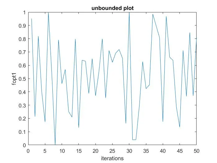
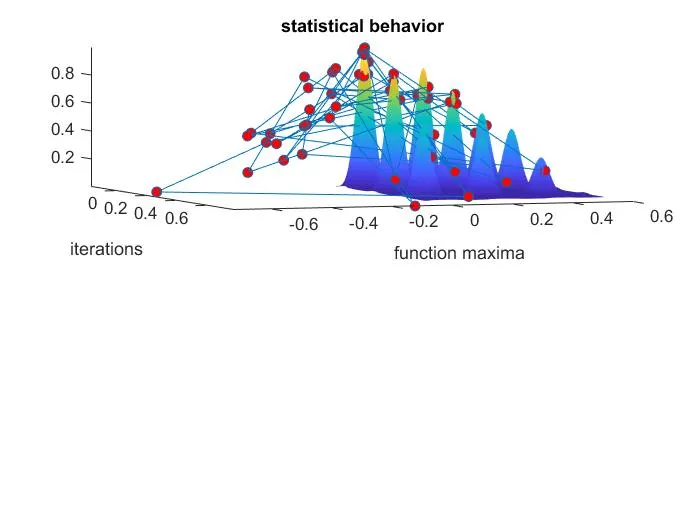
6. The first case of the study of the genetic algorithm provides the statistical behavior of the function apart from the mesh that is defined as seen by the plot generated.
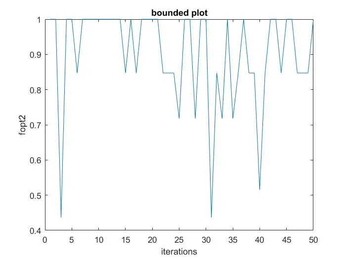
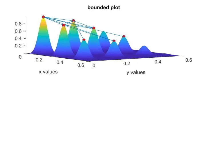
7. The second study will be done so that the genetic algorithm can be utilized in between the mesh grid provided, for that the syntax of genetic algorithm that has lower and upper bounds will be utilized in the program.
8. Since the program is still unable to give a fixed input of the value of the global maxima of the function the optimization of the function using the genetic algorithm function is used.
9. Each case study has an inbuilt plot generation command to monitor the number of iterations as well as fluctuations within the main program.
10. Each case study also has a timer command in them to calculate the time elapsed during the running of each individual case within the program.

Plots and contours:

• Case 1 Statistical behaviour of genetic algorithm
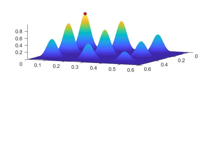
• Case 2 Statistical behaviour of the genetic algorithm with upper and lower bounds
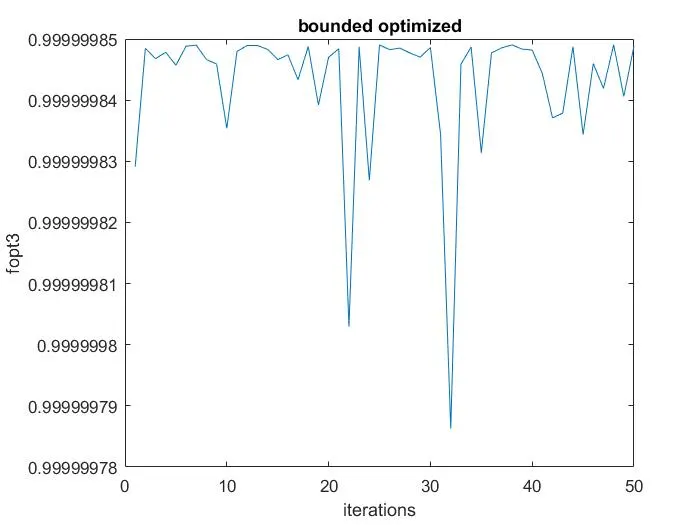
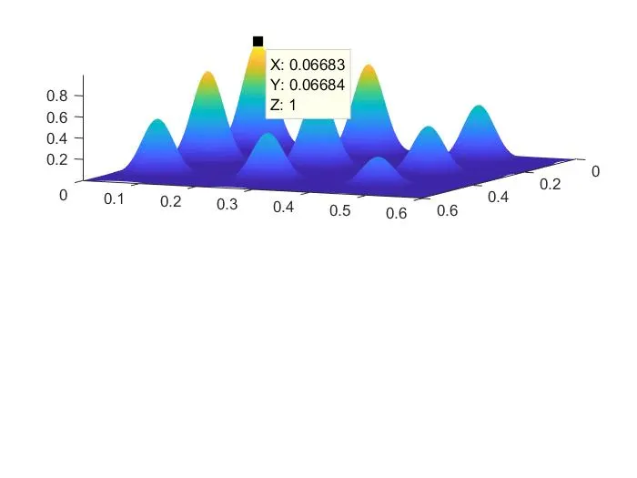
• Case 3 Optimized function

Errors and solutions:

• Apart from the syntax errors and use of the new commands like timer command no major errors occurred during the completion of the challenge.

Learning:

• Genetic algorithm

The following outline summarizes how the genetic algorithm works:

1. The algorithm begins by creating a random initial population.

2. The algorithm then creates a sequence of new populations. At each step, the algorithm uses the individuals in the current generation to create the next population. To create a new population, the algorithm performs the following steps:

   1. Scores each member of the current population by computing its fitness value.

   2. Scales the raw fitness scores to convert them into a more usable range of values.

   3. Selects members, called parents, based on their fitness.

   4. Some of the individuals in the current population that have lower fitness are chosen as elite. These elite individuals are passed to the next population.

   5. Produces children from their parents. Children are produced either by making random changes to a single parent—mutation—or by combining the vector entries of a pair of parents—crossover.

   6. Replaces the current population with the children to form the next generation.

3. The algorithm stops when one of the stopping criteria is met

• Syntax of GA command used in the report

The Genetic algorithm syntax given by the Matlab is as follows:

x=ga(fun,nvars,A,B,Aeq,Beq,LB,UB.nonlcon,intcon,options)

here,

fun=objective function

nvars= number of variables

A & B= subject to linear inequalities of the form A*x<=B

Aeq & Beq = subject to linear equalities of the form A*x=B

LB= Lower bound

UB= upper Bound

nonlcon= non-linear inequalities

intcon= integer constrained

options= Adds constraint tolerance by increasing the population size

• Same output even if the number of iteration is increased

The genetic algorithm uses the following conditions to determine when to stop:

• Generations — The algorithm stops when the number of generations reaches the value of Generations.

• Time limit — The algorithm stops after running for an amount of time in seconds equal to the Time limit.

• Fitness limit — The algorithm stops when the value of the fitness function for the best point in the current population is less than or equal to the Fitness limit.

• Stall generations — The algorithm stops when the average relative change in the fitness function value over Stall generations is less than Function tolerance.

• Stall time limit — The algorithm stops if there is no improvement in the objective function during an interval of time in seconds equal to the Stall time limit.

• Stall test — The stall condition is either average change or geometric weighted. For geometric weighted, the weighting function is 1/2ⁿ, where n is the number of generations prior to the current. Both stall conditions apply to the relative change in the fitness function over Stall generations.

• Function Tolerance — The algorithm runs until the average relative change in the fitness function value over Stall generations is less than Function tolerance.

• Nonlinear constraint tolerance — Nonlinear constraint tolerance is not used as a stopping criterion. It is used to determine the feasibility with respect to nonlinear constraints. Also, a point is feasible with respect to linear constraints when the constraint violation is below the square root of Nonlinear constraint tolerance.

The algorithm stops as soon as anyone of these conditions is met.

• Graph for three studies

1. In the first case study since there are no limits f thus the genetic algorithm does not search between the required values of 0 and 1, hence each execution of the program yields a different optimum value of the global maxima.
2. In the second case study since the lower and upper limits are included in the syntax of the genetic algorithm thus most of the values of the maxima in each iteration are obtained between 1 and 0.4. This method narrows down the maximum values to three values as shown in the plot.
3. In the third case, the global maxima obtained is accurate and is narrowed down to a value of 0.0668.

Conclusion:

The above program in MATLAB successfully optimizes the stalagmite function and also the global maxima of the function is generated.

Reference:

1. https://in.mathworks.com/help/gads/what-is-the-genetic-algorithm.html
2. https://in.mathworks.com/help/gads/some-genetic-algorithm-terminology.html
3. Matlab help and support for genetic algorithm.
4. https://ieeexplore.ieee.org/abstract/document/1043452/
5. https://www.researchgate.net/profile/Manish_Saraswat2/publication/258789666_Optimization_of_Function_by_using_a_New_MATLAB_based_Genetic_Algorithm_Procedure/links/5d368b51a6fdcc370a577ffd/Optimization-of-Function-by-using-a-New-MATLAB-based-Genetic-Algorithm-Procedure.pdf