Genetic algorithm using MATLAB to calculate global maxima of a stalagmite function
Genetic algorithm using MATLAB to calculate global maxima of a stalagmite function
AIM:
To optimize the stalagmite function and find the global maxima of the function.
THEORY:
Genetic Algorithm (GA) is a search-based optimization technique based on the principles of Genetics and Natural Selection. It is frequently used to find optimal or near-optimal solutions to difficult problems which otherwise would take a lifetime to solve. It is frequently used to solve optimization problems, in research, and in machine learning.
Optimization:
Optimization is the process of making something better. In any process, we have a set of inputs and a set of outputs.
Optimization refers to finding the values of inputs in such a way that we get the “best” output values. The definition of “best” varies from problem to problem, but in mathematical terms, it refers to maximizing or minimizing one or more objective functions, by varying the input parameters.
The set of all possible solutions or values which the inputs can take make up the search space. In this search space, lies a point or a set of points which gives the optimal solution. The aim of optimization is to find that point or set of points in the search space.
Genetic Algorithm:
A genetic algorithm (GA) is a method for solving both constrained and unconstrained optimization problems based on a natural selection process that mimics biological evolution. The algorithm repeatedly modifies a population of individual solutions. At each step, the genetic algorithm randomly selects individuals from the current population and uses them as parents to produce the children for the next generation. Over successive generations, the population "evolves" toward an optimal solution.
You can apply the genetic algorithm to solve problems that are not well suited for standard optimization algorithms, including problems in which the objective function is discontinuous, nondifferentiable, stochastic, or highly nonlinear.
The genetic algorithm differs from a classical, derivative-based, optimization algorithm in two main ways, as summarized in the following table.
| Classical Algorithm | Genetic Algorithm |
|---|---|
| Generates a single point at each iteration. The sequence of points approaches an optimal solution. | Generates a population of points at each iteration. The best point in the population approaches an optimal solution. |
| Selects the next point in the sequence by a deterministic computation. | Selects the next population by computation which uses random number generators. |
Genetic Algorithm syntax
ga |
Find minimum of function using genetic algorithm |
Syntax
x = ga(fun,nvars)
x = ga(fun,nvars,A,b)
x = ga(fun,nvars,A,b,Aeq,beq)
x = ga(fun,nvars,A,b,Aeq,beq,lb,ub)
x = ga(fun,nvars,A,b,Aeq,beq,lb,ub,nonlcon)
x = ga(fun,nvars,A,b,Aeq,beq,lb,ub,nonlcon,options)
x = ga(fun,nvars,A,b,[],[],lb,ub,nonlcon,IntCon)
x = ga(fun,nvars,A,b,[],[],lb,ub,nonlcon,IntCon,options)
x = ga(problem)
[x,fval] = ga(___)
[x,fval,exitflag,output] = ga(___)
[x,fval,exitflag,output,population,scores] = ga(___)
GA Motivation
Genetic Algorithms have the ability to deliver a “good-enough” solution “fast-enough”. This makes genetic algorithms attractive for use in solving optimization problems. The reasons why GAs are needed are as follows −
Solving difficulty problem
In computer science, there is a large set of problems, which are NP-Hard. What this essentially means is that even the most powerful computing systems take a very long time (even years!) to solve that problem. In such a scenario, GAs prove to be an efficient tool to provide usable near-optimal solutions in a short amount of time.
Failure of gradient-based methods
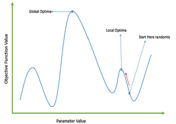
Traditional calculus-based methods work by starting at a random point and by moving in the direction of the gradient, till we reach the top of the hill. This technique is efficient and works very well for single-peaked objective functions like the cost function in linear regression. But, in most real-world situations, we have a very complex problem called as landscapes, which are made of many peaks and many valleys, which causes such methods to fail, as they suffer from an inherent tendency of getting stuck at the local optima as shown in the following figure.
Getting a good solution fast
Some difficult problems like the Travelling Salesperson Problem (TSP), have real-world applications like pathfinding and VLSI Design. Now imagine that you are using your GPS Navigation system, and it takes a few minutes (or even a few hours) to compute the “optimal” path from the source to destination. Delay in such real-world applications is not acceptable and therefore a “good-enough” solution, which is delivered “fast” is what is required.
PROCEDURE AND CODE EXPLANATION:
Stalagmite function:
Stalagmite function code:
- the stalagmite function is defined as the code given below:
function [f] = stalagmite(input_vector)
x = input_vector(1);
y = input_vector(2);

%To find the maxima end
f1_x = (sin(5.1*pi*x + 0.5)).^6;
f1_y = (sin(5.1*pi*y + 0.5)).^6;
f2_x = exp(-4*(log(2))*(((x - 0.00667).^2))./(0.64));
f2_y = exp(-4*(log(2))*(((y - 0.00667).^2))./(0.64));
f = -(f1_x*f2_x*f1_y*f2_y);    %conversion to maximization
end- A function (stalagmite) is created with the body of the function being the stalagmite equations and the function is multiplied with '-' in order to find the global maxima.
Program code:
Explanation:
- First defining the search space for x and y using 'linspace' command and giving the 'num_cases'.
- the 'mesh grid' command is used to create a two-dimensional mesh.
- The 'surfc' command is used to create a contour plot under the three-dimensional shaded surface.
- 'Shading interp' is used t0 make the plot smoother.
- 'Tic' and 'toc' commands are used to specify the start and end time intervals.
-
ga - Find minimum of function using genetic algorithm
The three study cases:
- Study 1: Unbounded input: Based on statistical behaviour.
- Study 2: Bounded input: Behaviour of upper and lower boundaries
- Study 3: Bounded with an increased population (At one point): Finding the global maxima.
clear all
close all
clc

%Defining our search space
x = linspace(0,0.6,150);
y = linspace(1,0.6,150);
num_cases = 50;

%Creating a 2-Dimensional mesh
[xx yy] = meshgrid(x,y);

%Evaluating the stalagmite function
for i = 1:length(xx)
    for j = 1:length(yy)
        input_vector(1) = xx(i,j);
        input_vector(2) = yy(i,j);
        f(i,j) = stalagmite(input_vector);
    end
end

figure(1)
hold on
surfc(xx,yy,-f)
xlabel('X values')
ylabel('Y values')
title('Stalagmite function')
shading interp
[inputs,fval] = ga(@stalagmite,2);


%STUDY:1 Statistical behaviour
tic
for i = 1:num_cases
    [inputs,fopt1(i)] = ga(@stalagmite,2);
    xopt1(i) = inputs(1);
    yopt1(i) = inputs(2);
end
study_time1 = toc;
figure(2)
subplot(2,1,1)
hold on
surfc(xx,yy,-f)
xlabel('X')
ylabel('Y')
shading interp

plot3(xopt1,yopt1,-fopt1,'marker','o','markersize',5,'markerfacecolor','r');
title('Unbounded inputs')
subplot(2,1,2)
plot(-fopt1)
xlabel('Iteratiom')
ylabel('Function_minimum')

%STUDY 2: Behaviour under upper and lower boundaries
tic
for i = 1:num_cases
    [inputs,fopt2(i)] = ga(@stalagmite,2,[],[],[],[],[0;0],[1;1]);
    xopt2(i) = inputs(1);
    yopt2(i) = inputs(2);
end
study_time2 = toc;
figure(3)
subplot(2,1,1)
hold on
surfc(xx,yy,-f)
xlabel('X')
ylabel('Y')
shading interp

plot3(xopt2,yopt2,-fopt2,'marker','o','markersize',5,'markerfacecolor','r');
title('bounded inputs')
subplot(2,1,2)
plot(-fopt2)
xlabel('Iteratiom')
ylabel('Function_minimum')

%STUDY 3: Increasing the population
options = gaoptimset(@ga);
options = gaoptimset(options,'populationsize',300);
tic

for i = 1:num_cases
    [inputs,fopt3(i)] = ga(@stalagmite,2,[],[],[],[],[0;0],[1;1],[],[],options);
    xopt3(i) = inputs(1);
    yopt3(i) = inputs(2);
end
study_time3 = toc;
figure(4)
subplot(2,1,1)
hold on
surfc(xx,yy,-f)
xlabel('X')
ylabel('Y')
shading interp

plot3(xopt3,yopt3,-fopt3,'marker','o','markersize',5,'markerfacecolor','r');
title('At one point')
subplot(2,1,2)
plot(-fopt3)
xlabel('Iteratiom')
ylabel('Function_minimum')
Results:
Stalagmite plot
Study 1: Unbounded Inputs
The number of lines over the maxima and minima all over the plot which is insignificant.
Study 2: Bounded Inputs
Under upper and lower bounds given, there are lesser lines formed.
Study 3: Bounded with an increased population (At one point)
Conclusion:
In this third study, The GA value is concentrated in one are/point which is known to be global maxima.