Curve Fitting

Curve fitness characteristics can be checked by calculating the errors at each data points and evaluating. Ideally error should be equal to zero.

1. How to make a curve fit perfectly?

A: A perfect fit is achieved when there is no error between original data points and data points obtained using curve fit.

2. How to get the best fit?

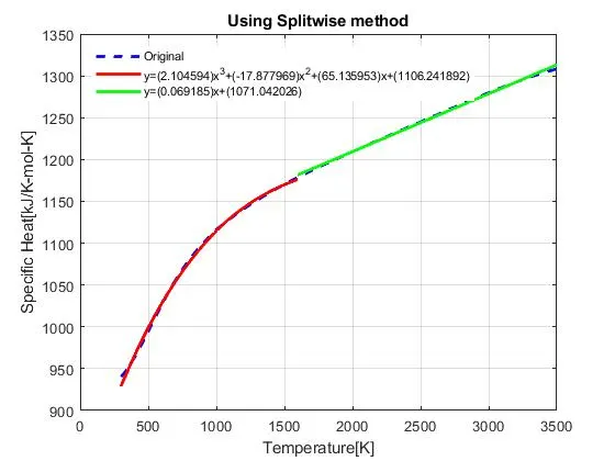
A: Best fit is achieved when the residual error is minimum. One of the methods to check this is by Root mean sqaure method(RMS). In matlab the best fit can be achieved by increasing the order of polynomials, spliting the data and fitting different polynomial curves.

3. What could be done to improve cubic fit?

A: Cubic fit can be improved by using centering and scaling to improve numerical properties. Doing this will centers the data at zero and scales it to have a standard deviation of 1, which avoid error while performing fit operation.

Output Images:

Figure(1): Linear & Cubic Plot

Figure(2): Using Splitwise method

MATLAB code:

close all
clear all
clc

%Load Input data
cp_data = load('data');
temperature = cp_data(:,1);
cp = cp_data(:,2);

%Linear Fit cp=a*T + c
coeff_linear = polyfit(temperature,cp,1);
pred_cplinear=polyval(coeff_linear,temperature);

%Cubic Fit cp=a*T^3 + b*T^2 + c*T+d
%Utilized centering and scaling to improve the cubic fit and remove warning
[coeff_cubic, S, mu] = polyfit(temperature,cp,3);
pred_cpcubic=polyval(coeff_cubic,temperature,S,mu);

%Plot original
figure(1)
plot(temperature,cp,'r--','linewidth',2,'color','b')
hold on

%Plot linear & cubic fit
plot(temperature,pred_cplinear,'linewidth',2,'color','r')
plot(temperature,pred_cpcubic,'linewidth',2,'color','g')
hold off

%Display grid
grid on

%Display title
title('Linear & Cubic plot')
%Display axis labels
xlabel('Temperature[K]')
ylabel('Specific Heat[kJ/K-mol-K]')

%To show linear & cubic equations in legend
equation_linear=sprintf('y=(%f)x+(%f)',coeff_linear(1),coeff_linear(2));
equation_cubic=sprintf('y=(%f)x^3+(%f)x^2+(%f)x+(%f)',coeff_cubic(1),coeff_cubic(2),coeff_cubic(3),coeff_cubic(4));

%Display legend
legend('Original',equation_linear,equation_cubic,'location','northwest','FontSize',7)



%2nd part of challenge Splitwise method of plotting 
%Based on obsrvation of original plot entire data set is divided into two
%Range 1 from 1 to 1301th term
%Range 2 from 1302 to end the term
temprange1=cp_data(1:1301,1);
temprange2=cp_data(1302:end,1);
cprange1=cp_data(1:1301,2);
cprange2=cp_data(1302:end,2);

%Fit a cubic polynomial from 1 to 1301th term
%Cubic Fit cp=a*T^3 + b*T^2 + c*T+d
[coeff_cubicrange1, S2, mu2] = polyfit(temprange1,cprange1,3);
pred_cpcubicrange1=polyval(coeff_cubicrange1,temprange1, S2, mu2);

%Fit a linear polynomial from 1302th term to end
%Linear Fit cp=a*T + c
coeff_linearrange2 = polyfit(temprange2,cprange2,1);
pred_cplinearrange2=polyval(coeff_linearrange2,temprange2);


figure(2)
%Plot curve fits using splitwise method
plot(temperature,cp,'r--','linewidth',2,'color','b')
hold on
plot(temprange1,pred_cpcubicrange1,'linewidth',2,'color','r')
plot(temprange2,pred_cplinearrange2,'linewidth',2,'color','g')
hold off

%Display grid
grid on

%Display title
title('Using Splitwise method')

%Display axis labels
xlabel('Temperature[K]')
ylabel('Specific Heat[kJ/K-mol-K]')

%To show linear & cubic equations in legend
equation_linearrange2=sprintf('y=(%f)x+(%f)',coeff_linearrange2(1),coeff_linearrange2(2));
equation_cubicrange1=sprintf('y=(%f)x^3+(%f)x^2+(%f)x+(%f)',coeff_cubicrange1(1),coeff_cubicrange1(2),coeff_cubicrange1(3), coeff_cubicrange1(4));

%Display legend
legend('Original',equation_cubicrange1,equation_linearrange2,'location','northwest','FontSize',7)