Week - 4 - Crash Box Simulation

OBJECTIVE: To simulate a crash test for the given FE model of a crash box using LS-Dyna. Request for the given deliverables and compare the results for a 1.2 mm thick and 1.5 mm thick crash box.

Deliverables ==>

- Input .k file and output files (d3plot, gistat, sleout, rcforc)

- Animation of the final simulation

- The cross-sectional force generated in the middle of the crash box (along its length)

- Acceleration plot of a node in the middle of the crash box (along its length)

- Maximum directional stress and strain along the length of the crash box (x strain, Y strain, etc)

- A plot of all energies (total, internal, kinetic, hourglass, sliding)

- Compare the accelerations and stress/strain plots of 1.2/1.5mm crash boxes.

INTRODUCTION:

A crash box is a highly energy-absorbing structure that crashes on the application of loads and reduces the impact on other components nearby. A full-fledges crash box is a highly sophisticated design but in this case, we will go with a rectangular channel which can be thought of as the most simple crash box.

Here are the different assumptions and information required:

- The crash box should crash into a rigid wall created using "RIGIDWALL_ keyword. Check the manual to understand and create a rigid wall.

- Material for the crash box is steel. The simulation needs to be started using elastic material to verify

its correctness and later a nonlinear material card data will be provided. The thickness of the crash box is 1.2mm.

- Initial velocity for the crash box should be around 50 kmph

- The units system to be used is gm-mm-ms

- The simulation should satisfy either of the two situations (1) It crashes on the rigid wall and rebounds completely or (2) it buckles and folds in the axial direction so as to come in self-contact.

- Once the simulation is completed and results are collected, run another simulation by increasing the thickness of the crash box from 1.2 to 1.5mm.

PROCEDURE:

1. Solver_deck set-up

i. Open the given FE model of the crash box in LSPP (Is-prepost).

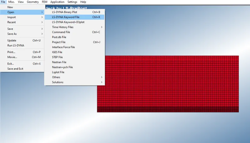
ii. The imported keyword file only contains a part. The rest of the details or properties of the part have not been defined. We need to define materials and sections for the crash box part and also set up a rigid wall for the crash test.

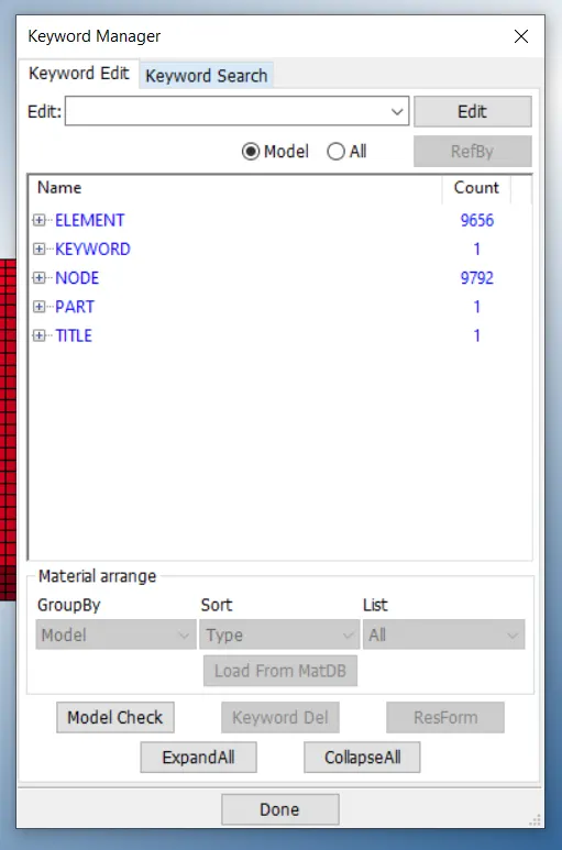
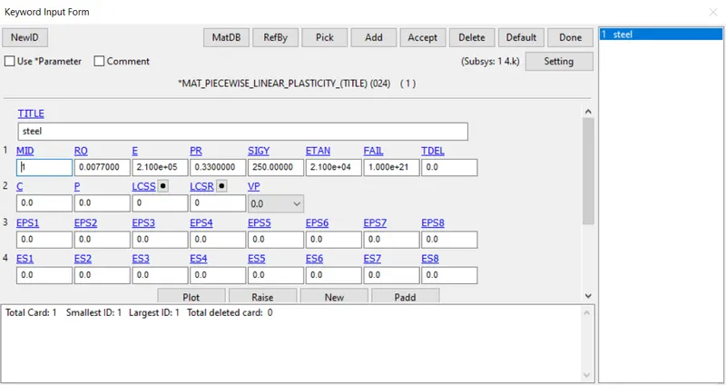
iii. First, we will try to complete the Part definition. Use the Keyword manager to open the part card. We will now create a *SECTION_SHELL_TITLE card and assign it to the part. While defining the section, the thickness to be assigned is 1.2 mm. For material, we will use the

*MAT_PIECEWISE LINEAR PLASTICITY_TITLE card for creating a material card for steel. Note: Extra care should be given to the units used. Here, we have been asked to use the g-mm-ms unit system. Thus, the E value for steel becomes 2.10E+5 MPa.

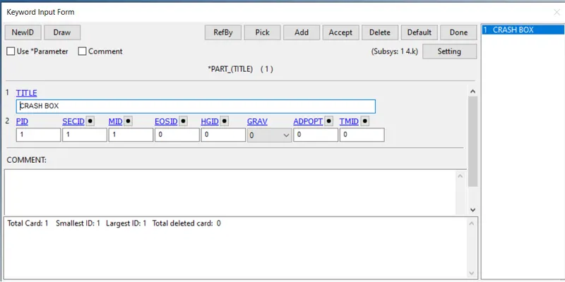
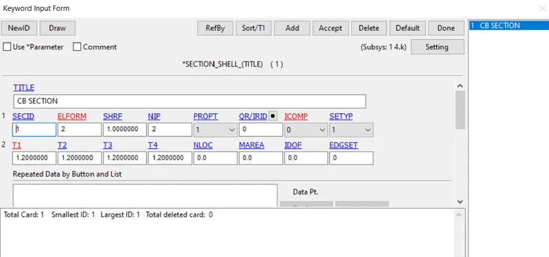
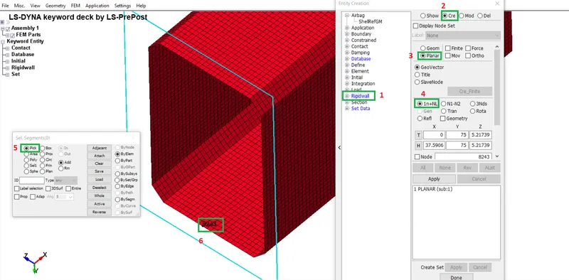
iv. Now we will create the Rigid wall using the create entity option. Note that the rigid wall can also be created using the Keyword manager("RIGIDWALL PLANAR ID card),

to create a rigid wall goto create entity >> 1.rigidwall >>2.create>>3.planer (as we want rigid wall as a plane)>>4. 1n+NL (by this we can define a node and normal direction of a node in a single click )>>5. pick>>6.pick a node where we want the wall to be.

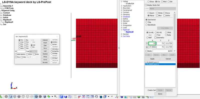
once we pick the node a rigid wall will be shown up. we have to give some distance to this wall from the model, we have given a distance of 10 mm in negative x-direction as shown below.

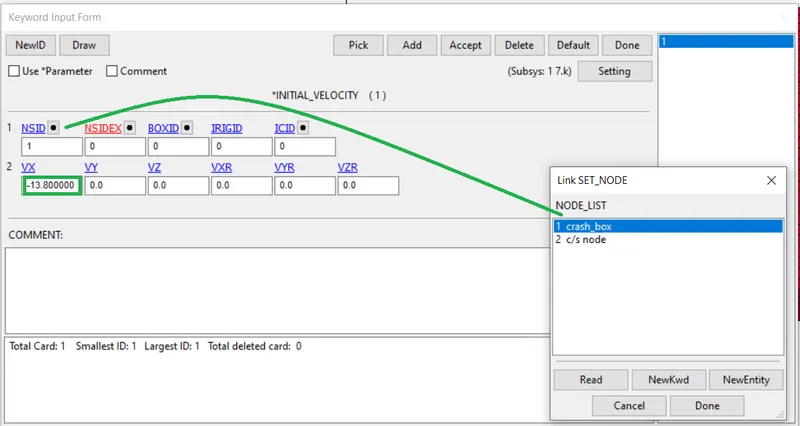
v. Now we need to define an initial velocity to the crash_box so that it impacts the created rigid wall. We have been asked to set the Initial velocity as 50Kmph which converts into 13.8 mm/ms ( i.e. 50*1000*(1000) / 3600000 = 13.887 mm/ms ). This initial velocity can be applied by using the Keyword manager and creating an "INITIAL_VELOCITY card with X-velocity as 13.8 mm/ms. Note that the initial velocity can also be assigned from the Create entity panel.

for defining initial velocity we are gonna need node set defined for entire crash box , and input velocity in respective direction

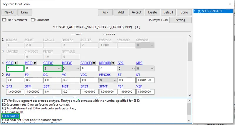
vi. We need to define self contact for the crash box. We will use the Keyword manager and create a *CONTACT AUTOMATIC_SINGLE_SURFACE_ID card to define it.

as we have created a rigid wall directly (i.e. we don't use any meshed shell as a rigid wall ) we don't need to define contact between wall and crash box

a contact is a method where were we select one surface as slave and another one as master, the slave is one where we want to know unknown values.it creates damping in the imaginary thickness around the slave component, when node from master component tries to penetrate the slave surface, the slave provides appropriate damping resistance to that penetration

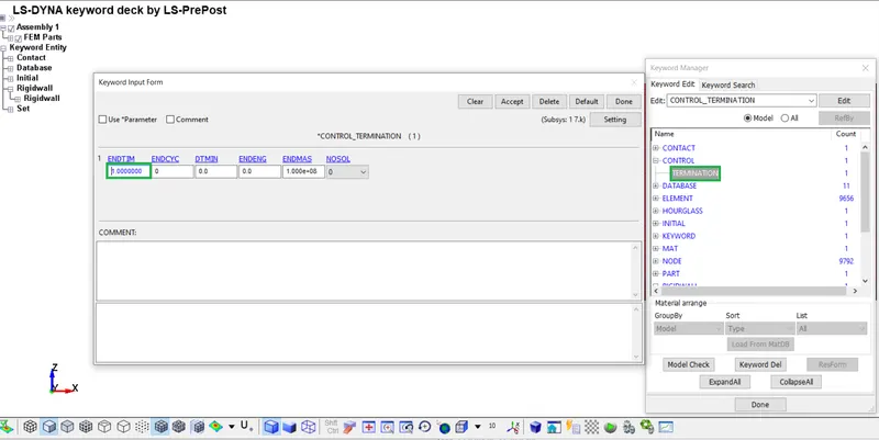
vii. Create a *CONTROL_TERMINATION card and set the runtime as 1 ms (i.e. V=D/T V=13.88,D=10 mm, T=? now T=0.72 ms ).

here we are taking 1 ms as we want to run the model for more time

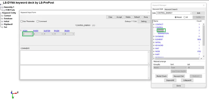
viii. To avoid Hourglass energy generation, we will create an *HOURGLASS card with ihq value as 2 and the rest as default. Now assign this Hourglass card to the Crash_box part.

note: previously we have defined keyword as hourglass but in here we didn't required that card as that card is only use where hourglass is more than 5% , , for hourglass calculation here we can use CONTROL >> ENERGY >> HGEN=2

ix. Now the solver deck set-up is complete. We need to run the analysis for 2 thicknesses, one 1.2mm and the other, 1.5 mm. The one that we have created here is for a 1.2 mm thick model. Thus we need to create another solver deck for the 1.5 mm thick model. This can be done very easily by simply changing the thickness value under the section definition in the Keyword file by opening it in Notepad. Then save it as a new file. We will do this after we have completed the total solver deck set-up including the Output requests as well.

Output_Request

i. Create output requests

using *DATABASE_GLSTAT, "DATABASE_MATSUM, DATABASE RCFORC, *DATABASE_RWFORC, "DATABASE SLEOUT, DATABASE_NODOUT and "DATABASE_BINARY_D3PLOT. Set 0.01 as the time interval between successive recorded values for all.

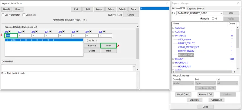
ii. We also need to plot the acceleration for a node midway the length of the crash box. For this, we will create 'DATABASE HISTORY_NODE using the create entity option and then create "DATABASE_NODOUT under the database ASCII for recording all the values related to this node (2468, in this case).

ENTER the node in ID1>>INSERT >>ACCEPT

iii. We also need to find the section force at a section midway the length of the crash box For this, we will create a section using *DATABASE- CROSS SECTION_SET for this we require a node set ID around section and Shell set ID as shown below.

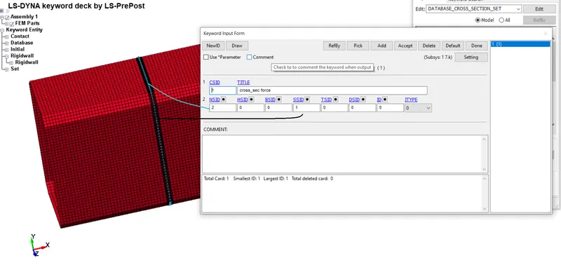
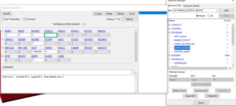
and then set "DATABASE - ASCII -SECFORC 0.01 to record all the values related to the created section.we also required *database-Extend_binary and in this card we have to give STRFLG as 1 and rest as default (this will allow us to plot stresses and strains in the section )

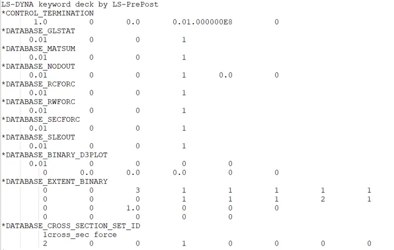
all the database requests are as shown below

iv. Now the solver deck setup is complete and ready to run the Analysis. We need to run the analysis for 2 thicknesses, one 1.2mm and the other, 1.5 mm. The Solver deck that we have created here is for a 1.2 mm thick model. Thus we need to create another solver deck for the 1.5 mm thick model. This can be done very easily by simply changing the thickness value under the section definition in the Keyword file by opening it in Notepad. Then save it as a new file.

for 1.5 mm thickness.

RESULTS OF ANALYSIS

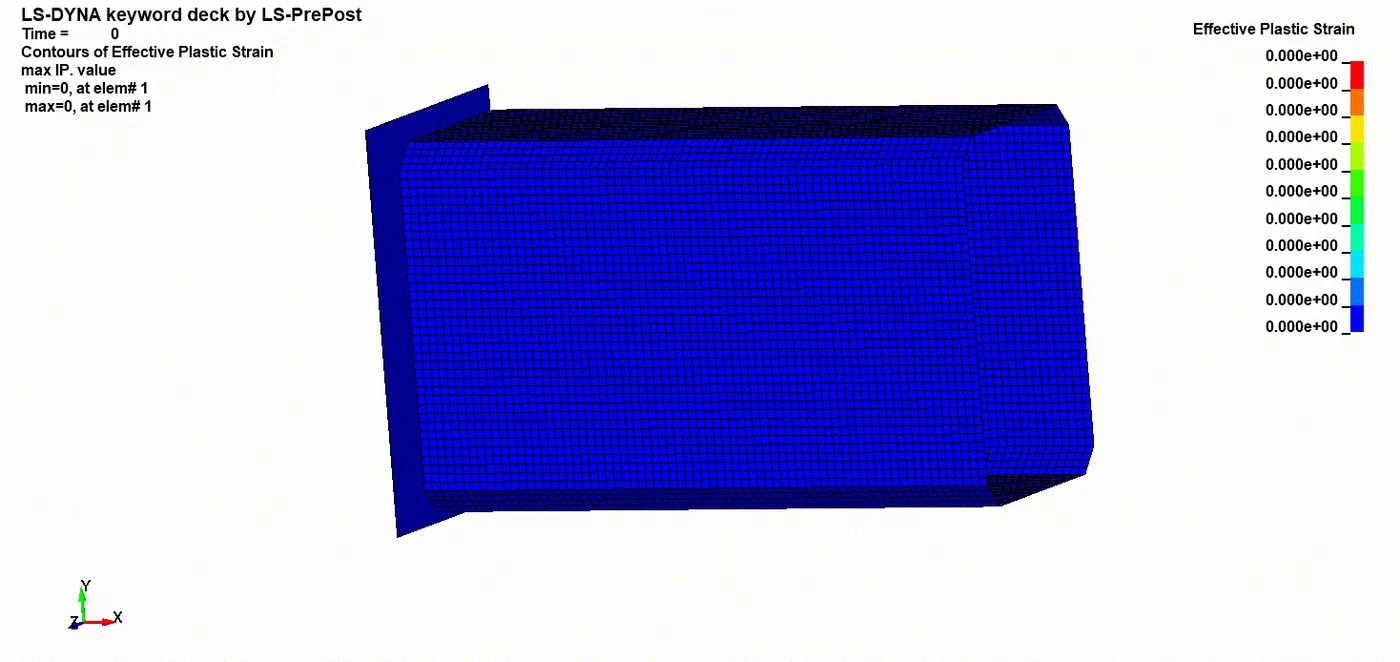
below is animation file recorded from file >> movie >> gif >>start give visual representation of strains in 1.2 mm crash box.

sectional forces

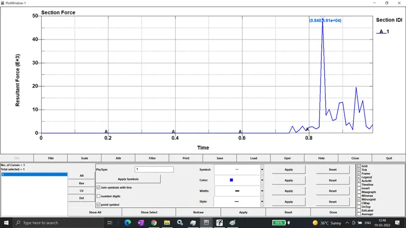
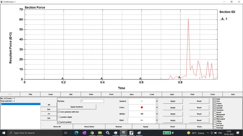
from it can be understood that there is not much difference in force behaviour in both of the cases except of in magnitude at around 0.74 ms both model hits the wall and at 0.84 ms second both section reaches their highest value the max force experienced in case 1 is 4.91e+04 while in case two with 1.5 thickness their force experienced is 6.15e+04 which is higher than case 1

The sectional forces are zero until the impact happens. On impact, the force can be seen to have suddenly increased to its peak value. Thereafter, the force gets reduced and oscillates which is due to vibration after impact .

Accelaration plot (at node 2468):

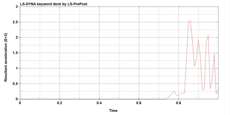
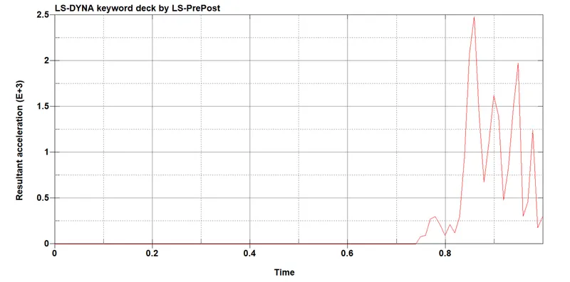
in acceleration up to 0.74 milisecond acceleration is zero as velocity is constant , as model hits it acceleration changes, maximum acceleration attained in case 1 is slightly higher than case 2 , after initial hit there is peak acceleration and then there are some rises in acceleration but each next peak acceleration is lower than before.

global energies:

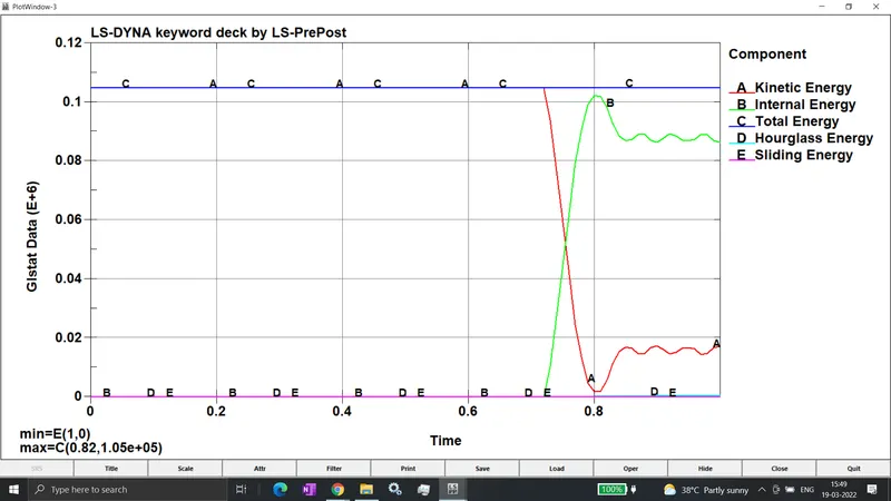
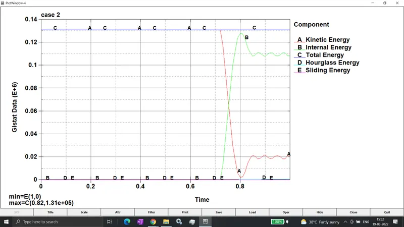
The Global Energy plots show the Kinetic energy, internal energy, Total energy, Sliding energy, and Hourglass energy values for the crash simulation.

The Energies are higher for the 1.5 mm thick crash box. The total energy for the 1.2 mm thick and 1.5 mm thick crash box was recorded as 1.05e+05 N-mm and 1.31e+05 N-mm respectively.

At 0 ms, the whole of the total energy is Kinetic energy. But as the simulation progresses and the impact between the Crash box and the Rigidwall takes place, at approx 0.74 ms, the Kinetic energy starts getting converted into Internal energy. The Internal energy reaches its peak and the kinetic energy reaches its lowest value at about 0.80 ms when the crash box is on the verge of getting rebounded from the rigid wall. The crash box then moves with a constant rebound velocity which is reflected in the energy plot as internal energy gets converted to kinetic energy and remains constant through the rest of the simulation.

stress and strain plots along directions

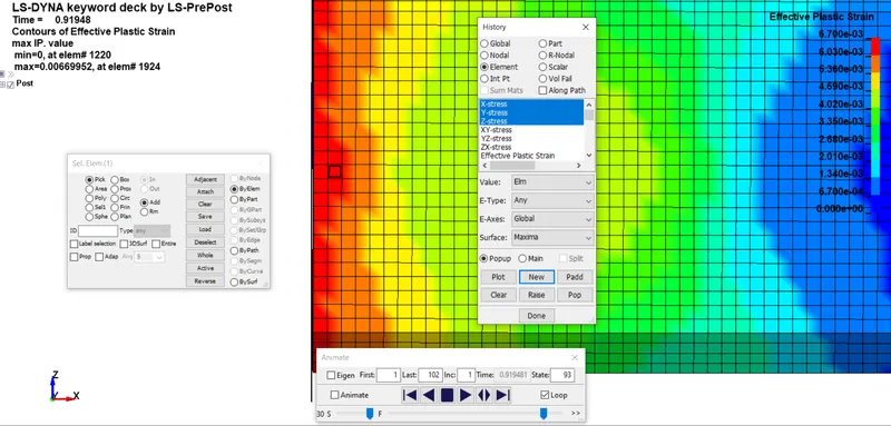
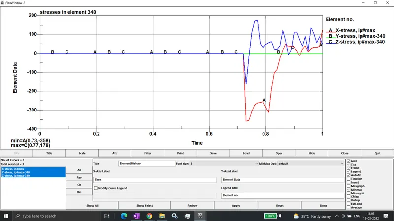
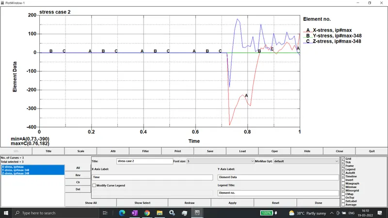
in both cases, the stresses in x directions (compression stress) are greater and in both cases magnitudes, case 2 magnitudes are high. stresses in z direction are comparatively less that is tension stress, stresses in y-direction are zero

strain plot

stain plots at element s348

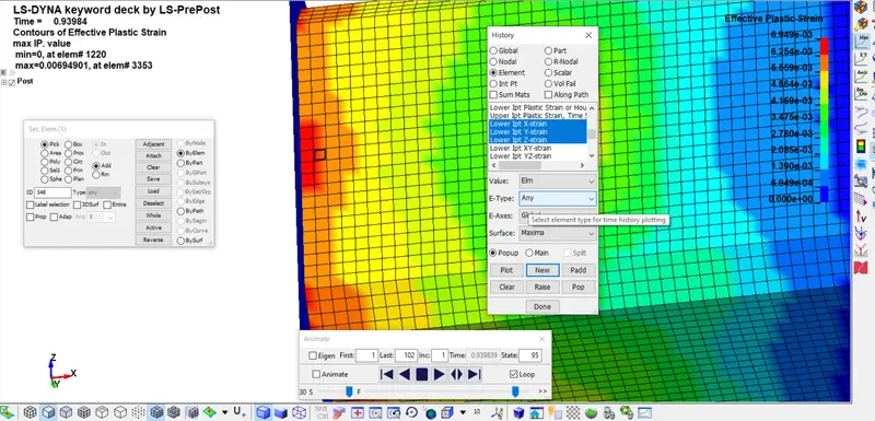
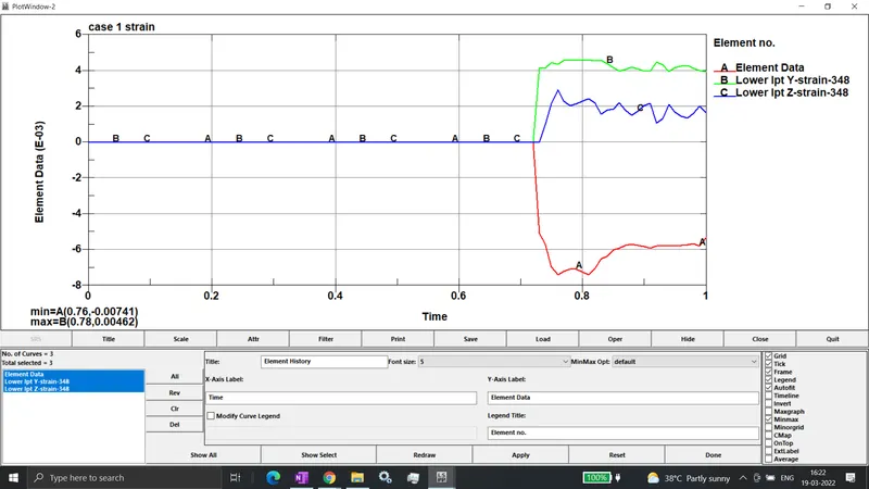
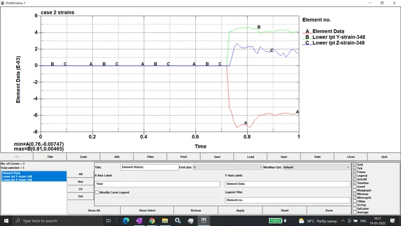
from the graph we can see that most of the straining happens in x direction that is compression strain , both y and z directions have some tension stains

CONCLUSION:

i. The solver deck was set-up for the crash simulation and the required results were requested using the appropriate *DATABASE keyword cards.

ii. The analysis ran successfully. Post-processing of the results was done using the D3plots and the other output ASCII result files, to produce the deliverables.