Week 4 - Combustion Efficiency Calculation after Preheating

INTRODUCTION

The most important method by which power is generated is by burning fossil fuels. Burning or combustion is a process where the hydrocarbon fuels reacts with oxygen in the atmospheric air and generates heat as well as other products of combustion.The combustion of fossil fuels results in the generation of heat energy which used for the generation of electricity, the methods in which the electric power is generated depends on the powerplant. But it is very important to note that a large amount of heat generated while combustion is wasted with the flue gases. So to utilize that heat energy wasted with the flue gases, the flue gases is used to preheat the incoming air which is used for combustion of the fuel.

It is important to note that the Adiabatic flame temperature depends on the temperatures of the reactants, so if the initial temperature of the air is changed by preheating the adiabatic flaame temperature also changes. The effect of preheat on AFT and the combustion efficiency can be analysed using the cantera module in python. It is important to note that fuel can be saved by preheating since a reasonable amount of heat energy is saved when the heat energy of the flue gases are used.

AIM

The aim of this project is to study the effect of preheating on adiabatic flame temperature and also its effect on the fuel efficiency.

The preheating temperature is varied between 298 and 600K,

RESULTS AND DISCUSSION

The code for determining the effect of preheating on the AFT is given below:

import cantera as ct
import matplotlib.pyplot as plt
import numpy as np

gas = ct.Solution('gri30.cti')

# Methane fuel

fuel = ct.Quantity(gas)
fuel.TPX =298,ct.one_atm,{'CH4':1}
fuel.moles =1

#Air
T_min = 298
T_max = 600
N = 20

air =ct.Quantity(gas)
Temp_air = np.linspace(T_min,T_max,N)

for Temp in Temp_air:
    air.TPX = Temp,ct.one_atm,{'O2':0.21,'N2':0.79}
    air.moles = 2/0.21
    M = fuel + air 
    M.equilibrate('HP','auto')
    plt.plot(Temp,M.T,'-o',color='red')
    

plt.title('Effect of preheating on the Adiabatic Flame Temperature(AFT) of $CH_4$')
plt.xlabel('Preheating Temperature (K)')
plt.ylabel('Adiabatic flame Temperature (K)')
plt.grid(True)
plt.show()

The stepwise explanation of the above code is as shown below:

import cantera as ct
import matplotlib.pyplot as plt
import numpy as np

In the above snippet of code the required libraries are imported.

gas = ct.Solution('gri30.cti')

# Methane fuel

fuel = ct.Quantity(gas)
fuel.TPX =298,ct.one_atm,{'CH4':1}
fuel.moles =1

The variable is an instance of the solutions class, fuel is defined as the instance of the Quantity class. The initial temperature, pressure and the mole fraction of the fuel is initialised using the fuel.TPX command. The number of moles of fuel is set as 1.

#Air
T_min = 298
T_max = 600
N = 20

air =ct.Quantity(gas)
Temp_air = np.linspace(T_min,T_max,N)

for Temp in Temp_air:
    air.TPX = Temp,ct.one_atm,{'O2':0.21,'N2':0.79}
    air.moles = 2/0.21
    M = fuel + air 
    M.equilibrate('HP','auto')
    plt.plot(Temp,M.T,'-o',color='red')
    

The preheat temperature of the air is varied between 298 and 600 K. The initial temperature is varied using a for loop and the mixture is created using the quantity class to calculate the adiabatic flame temperature. The AFT as a function of the preheat is plotted using the plot() function in the pyplot module of the matplotlib library.

plt.title('Effect of preheating on the Adiabatic Flame Temperature(AFT) of $CH_4$')
plt.xlabel('Preheating Temperature (K)')
plt.ylabel('Adiabatic flame Temperature (K)')
plt.grid(True)
plt.show()

The title, xlabel, ylabel etc. for the plot is specified using the above snippet of code. The output of the above code is given below:

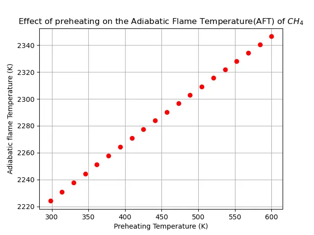
From the above picture it can be seen that the AFT increases as the preheat is increased.

The effect of preheating on the efficiency of the reaction is analysed using the following code. The LHV of the fuel is assumed to be to be 50MJ/kg. The exit temperature of the products are set to be 1700K and the products of combustion are assumed to be `CO_2, H_2O and N_2`.

The reaction can be written as `CH_4 + 2(O_2 + 3.76N_2) -> CO_2 + 2H_2O + 7.52N_2`. From this it can be seen that the number of moles of air = 9.52 and the number of moles of the product is 10.52. The mole fraction of `CO_2` can be calculated as `\chi_{CO_2}= \frac{1}{10.52}=0.095` similarly `\chi_{H_2O}= \frac{2}{10.52}=0.1901` and `\chi_{N2}= \frac{7.52}{10.52}=0.7148`

The heat released after the combustion can be calculated using the formula given below:

`Q_r = \dot{m}_f\timesh_f + dot{m}_a\timesh_a - (\dot{m}_f +\dot{m}_a)\timesh_p`

where the subscripts `f,a \& p` represents the fuel, air and the products of combustion respectively.

The theoretical heat supplied can be calculated to be:

`Q_s =m_f\times LHV`

The efficiency `\eta =\frac{Q_r}{Q_s}` = `\frac{\dot{m}_f\timesh_f + dot{m}_a\timesh_a - (\dot{m}_f +\dot{m}_a)\timesh_p}{\dot{m}_f\timesLHV`

which we can write as `eta = \frac{h_f + dot{m}_a/\dot{m}_f\timesh_a - (1 +\dot{m}_a/\dot{m}_f)\timesh_p}{LHV}` and `\dot{m}_a/\dot{m}_f = AF` the air fuel ratio.

So we can write

`eta = \frac{h_f + AF\timesh_a - (1 +AF)\timesh_p}{LHV}`

The code is given below:

import cantera as ct
import matplotlib.pyplot as plt
import numpy as np

gas = ct.Solution('gri30.cti')

# Methane fuel

fuel = ct.Quantity(gas)
fuel.TPX =298,ct.one_atm,{'CH4':1}
fuel.moles =1
mass_fuel = fuel.mass

# Products of combustion

products = ct.Quantity(gas)
products.TPX = 1700,ct.one_atm,{'CO2':0.095,'H2O':0.1901,'N2':0.7148}
products.moles =10.52
mass_product = products.mass


#Air
T_min = 298
T_max = 600
N = 20
LHV = 50e6

air = ct.Quantity(gas)
Temp_air = np.linspace(T_min,T_max,N)

for Temp in Temp_air:
    air.TPX = Temp,ct.one_atm,{'O2':0.21,'N2':0.79}
    air.moles = 2/0.21
    mass_air = air.mass
    
    h_air = air.enthalpy_mass
    h_fuel = fuel.enthalpy_mass
    h_products = products.enthalpy_mass
    
    AF = mass_air/mass_fuel
    
    Q = AF*h_air + h_fuel - (AF+1)*h_products
    
    Qs = LHV
    
    eta = (Q/Qs)*100
    
    plt.plot(Temp,eta,'*',color='red')
    
    
    
    
   
plt.grid()
plt.xlabel('Preheating Temperature (K)',fontsize =14)
plt.ylabel(r'Efficiency $\eta $ (%)',fontsize=14)
plt.title('Efficiency v/s Preheating Temperature',fontsize = 16)
plt.savefig('effvspheat.png')
plt.show()

The stepwise explanation of the codeis shown below:

import cantera as ct
import matplotlib.pyplot as plt
import numpy as np

In the above snippet of code the required libraries are imported.

gas = ct.Solution('gri30.cti')

# Methane fuel

fuel = ct.Quantity(gas)
fuel.TPX =298,ct.one_atm,{'CH4':1}
fuel.moles =1
mass_fuel = fuel.mass

# Products of combustion

products = ct.Quantity(gas)
products.TPX = 1700,ct.one_atm,{'CO2':0.095,'H2O':0.1901,'N2':0.7148}
products.moles =10.52
mass_product = products.mass

In the above snippet of code, gas is an instance of the solutions class. The fuel and the products are initialised the conditions as explained before.

#Air
T_min = 298
T_max = 600
N = 20
LHV = 50e6

air = ct.Quantity(gas)
Temp_air = np.linspace(T_min,T_max,N)

for Temp in Temp_air:
    air.TPX = Temp,ct.one_atm,{'O2':0.21,'N2':0.79}
    air.moles = 2/0.21
    mass_air = air.mass
    
    h_air = air.enthalpy_mass
    h_fuel = fuel.enthalpy_mass
    h_products = products.enthalpy_mass
    
    AF = mass_air/mass_fuel
    
    Q = AF*h_air + h_fuel - (AF+1)*h_products
    
    Qs = LHV
    
    eta = (Q/Qs)*100
    
    plt.plot(Temp,eta,'*',color='red')
    
    
    
    
   
plt.grid()
plt.xlabel('Preheating Temperature (K)',fontsize =14)
plt.ylabel(r'Efficiency $\eta $ (%)',fontsize=14)
plt.title('Efficiency v/s Preheating Temperature',fontsize = 16)
plt.savefig('effvspheat.png')
plt.show()

In the above snippet of code, the preheating of air is achieved by setting the initial temperature which is changed using a for loop. For every value of the preheat, the efficiency is calculated in the for loop. The matplotlib library is used to plot the efficiency v/s temperature graph. The output of the above code is shown below.

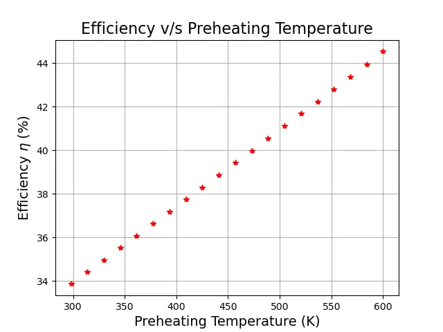
From the above image it is clear that as the preheat temperature increases, the efficiency also increases. It is also important to note that the exit temperature of the furnace is kept as 1700K. It is important to control the exit temperature since excessive high temperature can damage the furnace.

It is very important to note that the exit temperature from the furnace must be constant or in other words a fixed value. The value depends on many factors including the material properties. It is a correct practice of fixing the exit temperature.

CONCLUSION

It can be seen that as the preheating is increased, the AFT also increases. It is also important to note that the efficiency of the combustion process also increases with the preheating temperature.