Project Report

Introduction

CHT or conjugate heat transfer, refers to a heat transfer process involving an interaction of conduction within a solid body and the convection between the moving liquid media and solid media. Heat transfer in the solid domain is primarily due to conduction, for the fluid domain, it is dominated by convection. The heat transfer from one media to other, depends upon the fluid particles velocity to some extent.

There is a wide range of application of the CHT phenomenon, most primarily in cooling applications. A wide variety of active as well as passive cooling systems is employed around the heat producing electric or mechanical component, that works on CHT phenomenon. One of the common live examples around us is fins for circuit board, using natural convection or passive cooling.

CHT analysis plays a crucial role in determining the products design. As a rule of thumb, increased surface area leads to faster cooling, but the exact dimensions have to be simulated in order to be applied effectively. CHT analysis is very handy and important method with which can calculate the design parameters and reveal important data points before experimentation.

Objectives

Simulate CHT in a vehicle exhaust manifold, in order to calculate wall heat transfer coefficient. Also, Walkthrough to the tubulence modelling approach, by using K-epsilon and K-omega SST models.

Outline of the Study

In order to achieve the objective, the study has been outlined in the order of baseline simulation, followed by grid independence then meshing the boundary layer followed up by the simulation for heat transfer coefficient, temperature profile and other required physical parameters.

1. Baseline Simulation

The computation model is run with the default meshing (Ansys Mesher Module), with the required boundary conditions, inlet, outlet and convection. In this model, the minute details like wall heat transfer coefficients are not calculated, as the results might not be relevant with default mesh.

The sole purpose of the baseline simulation is to have a general idea about the computational complex zones and need for mesh refinement. With the insights of the baseline simulation, further grid independence analysis is done.

2. Grid Independence

Grid Independence for fluid zone followed up by solid zone is performed. Surface averaged Temperature and velocity at the outlet is used as a control variable mesh refinement of fluid zone.

Surface averaged temperature at the convection surface is used as a control variable for the mesh refinement for solid region.

Body sizing of the solid and fluid is zone is varied in order to observe the change in control variables. For the mesh refinement of fluid zone, the element size of solid region is kept constant and vice versa. The study is further followed by simulation for the desired physics.

3. Simulation using the refined mesh

The refined mesh is further modified for the boundary layer calculations. Since we are dealing with simulating the boundary layer physics, the viscous layers need to be refined with application of proper turbulence model, or it has to be approximated by appropriate wall function.

In order to simulate using different Turbulence models, two cases have been designed: -

Case 1: -

Velocity around the viscous layer has great contribution in the wall heat transfer coefficient calculation. So, in the present case, Y+ will be aimed at 1. Viscous layer resolution strategy has been used for resolving boundary layer phenomenon.

The K-omega SST model has been used to model the viscous flow.

Since, fluid medium is air, `mu = 1.79X10^-5 {kg}/{m.s}`, `rho = 1.225 {kg}/{m^3}`

Velocity of 5m/s is used in the calculation of first cell height.

Diameter of the pipe is measured to be about 15 mm

Calculation of Fist Layer Thickness: -

Renolds No. Calculation(Re) – `{rho*U*D}/{mu}` = 5132.68

Skin Friction Calculation(`C_f`) – `0.079 X Re^{-0.25}` = 0.00933

Wall Shear Stress – `tau_w = 0.5 * C_f * rho * U^2` = 0.14286kg/(m.s^2)

Frictional Velocity – `U_t = sqrt({tau_w}/{rho})` = 0.341m/s

First Layer Thickness as per selected y+ = `{y^+ *mu}/{rho*U_t}` = 0.00004m

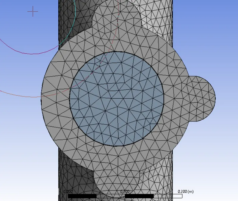
Inflation Layers

Case 2: -

For Instance, if the computation would be too heavy to carry out with mesh resolution in the vicinity of boundary layer, then the wall function approach may be used which will approximate the near wall phenomenon with empirical equation with K-epsilon model with enhanced wall treatment. This strategy is more common for industrial applications, as it reduces the element density hence, reduces the computational resource to arrive a solution.

In order to approximate the phenomenon around the wall, Y+ of 30 will be used to calculate the first layer thickness.

Calculation of Fist Layer Thickness: -

using above data,

First Layer Thickness as per selected y+ = 0.00128m

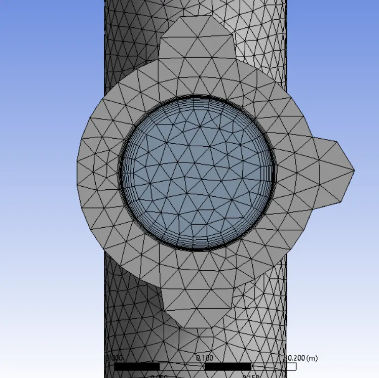
Inflation Layers

Mesh Refinement

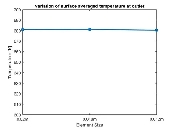
Surface Averaged Temperature at outlet with decreasing element size.

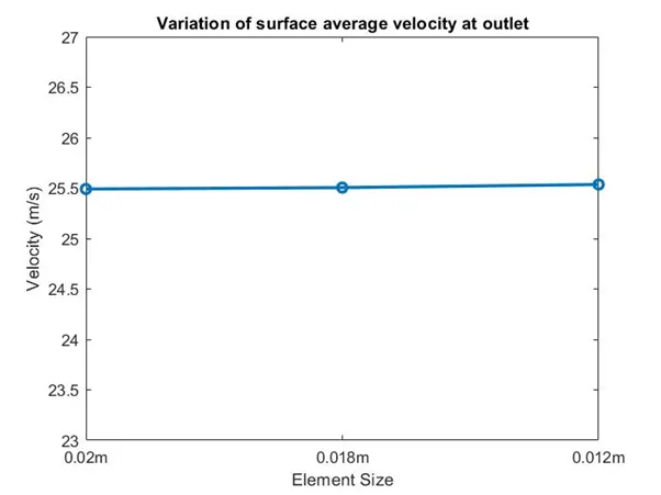
Surface Averaged Velocity at outlet with decreasing element size.

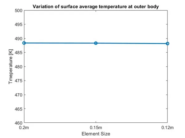
Surface Averaged Temperature at outer-wall-convection boundary with decreasing element size.

As per the observation, its clear that there is no appreciable change in computed values with change in mesh. So element size of 0.2m has been used for outer solid domain and 0.018m has been used for the fluid domain.

Solution Methodology

Ansys has been used in formulating the problem and solve the computational model. The geometry of the exhaust manifold has been adopted from the source provide. Later in Ansys SpaceClaim the geometry has been modified following meshing and solving as discussed below.

Geometry

The cad file of exhaust file was imported from the source provided. Ansys SpaceClaim has been used to preprocess the geometry for setting up computational domain.

At first fluid region is defined using Volume Extract method in SpaceClaim. After that, geometry is checked for Overlapping bodies, following the topology is shared between solid and fluid domain. Overlapping and topology share has been achieved by available method is SpaceClaim -> Workbench.

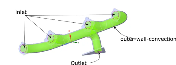
The geometry and boundary names are depicted in the picture below.

Meshing

Ansys Meshing module has been used to generate the computational mesh. Since the geometry has solid and fluid domains, body sizing of fluid and solid domain has been done for effective meshing. Also, we are interested in boundary layer phenomenon so inflation layer has been added for the same.

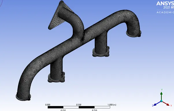
Overall Mesh of the body

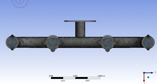
Mesh in the inlet section.

Though Mesh Refinement has been done in the present study, it doesn’t claim to be the perfect mesh for this type of simulation. The constrain of ANSYS academic license restricts more than 512000 elements/nodes in the computational problem.

Boundary Condition

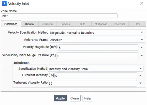
Inlet is subjected to velocity-inlet type boundary condition the temperature of air is set to 700K.

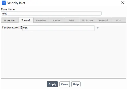
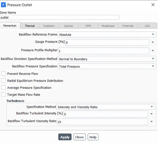
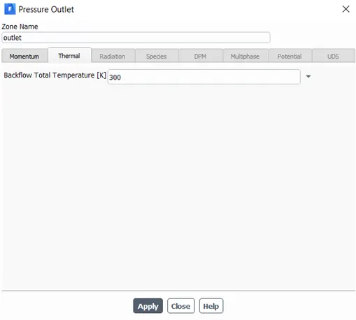
Outlet has gauge pressure of 0 and backflow temperature of 300K.

The outer-wall-convection has been subjected to convection with a heat transfer coefficient of 20W/(m2K).

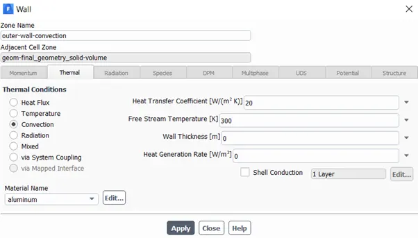
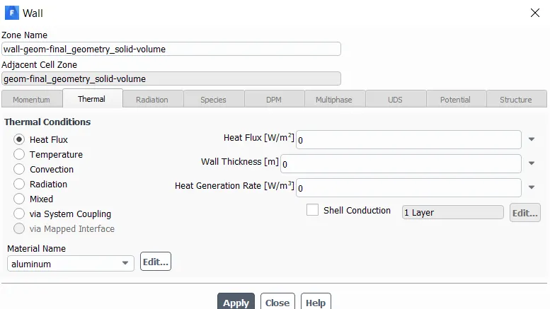
The flanges are given adiabatic boundary conditions, by making heat flux 0.

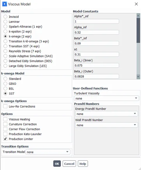
Viscous Model

Case 1

K omega SST has been used to model the turbulent flow.

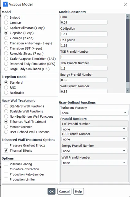
Case 2

K epsilon with enhanced wall Treatment

Results and Discussion

Case 1

Residual

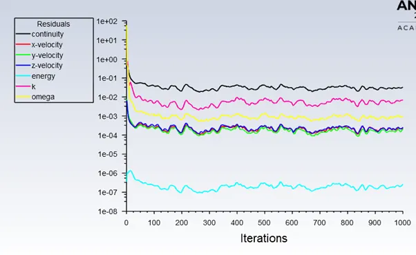
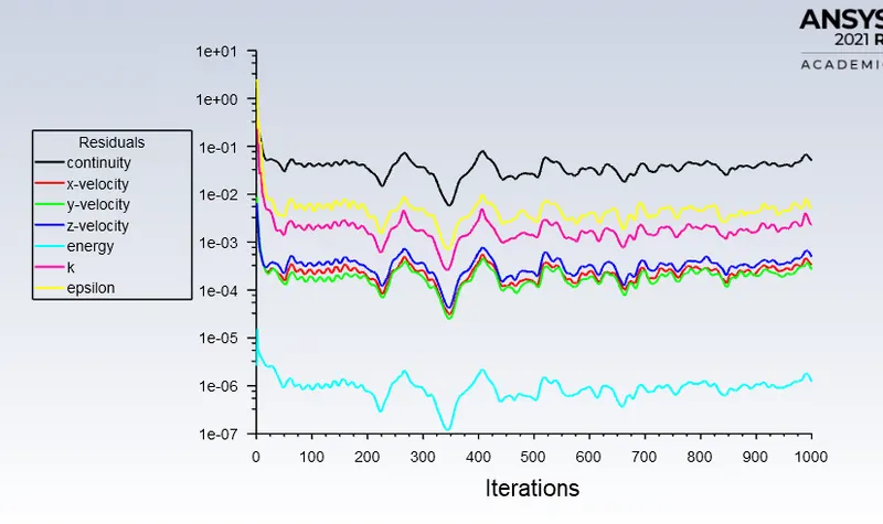
On observing the residual plot, it dont seem to diverge over iterations, also the amplitude of increase-decrease residuals diminishes which describes it convergence charactericts.

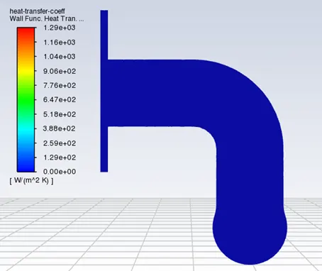
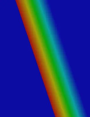
Wall Heat Transfer Coefficient - Contour Plot

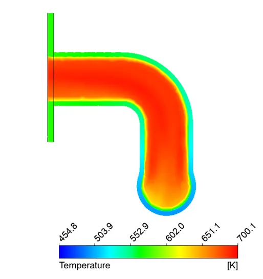
Temperature Contour Plot of the exhaust pipe

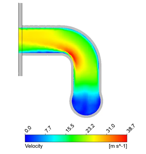
Velocity Contour Plot of the Exhaust Pipe

Case 2

Residual Plot

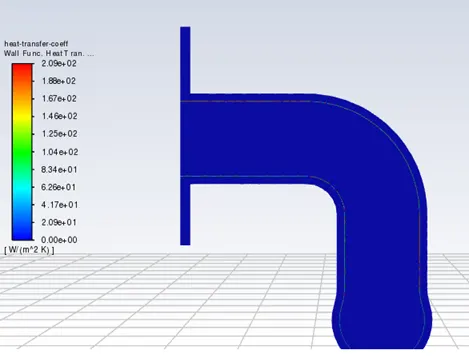
Heat Transfer Coefficient Plot

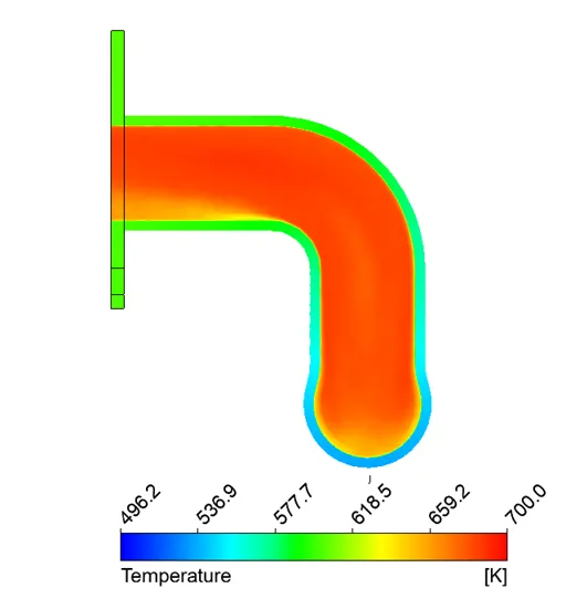
Temperature Contour Plot over the exhaust pipe

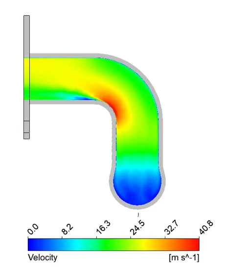
Velocity contour plot on exhaust pipe.

Conclusions:-

Validity of the simulation results:-

Heat Transfer Coefficient calculation is a function of temperature gradient as well as heat flux. Which is indirectly related to the flow velocity. Since the velocity is increased in the neck region of the outlet, the heat transfer coefficient has increased.

Also, Nusselt Number is a function of renolds no and prandlt number. Also, Heat Transfer Coefficient is function of nusselt number. This also elaborates the increased HTC around the increased velocity region.

Factors affecting the calculation:-

Inflation Layer: - The no. of layers should be increased around the high velocity region, it will help to resolve the boundary layer to a good factor.

Mesh Density in viscininty of Fluid - Solid Contact :- The mesh density should be high around the region for a better heat transfer calculation and reducing the averaging of temperature field.

Reduction of element size: - After increrase in the surface mesh density between solid liquid interface, there would be need of increase in no. of elements in both fluid and solid domain.

Better Inflation Layer: - The inflation layer should not be of same height all over the interface. It should be choosen as per the velocity in the viscinity of the interface.