Week 4 - CHT Analysis on Exhaust port
Conjugate Heat Transfer
Conjugate heat transfer corresponds with the combination of heat transfer in solids and heat transfer in fluids. In solids, conduction often dominates whereas in fluids, convection usually dominates. Conjugate heat transfer is observed in many situations.
Why CHT analysis is used?
Conjugate heat transfer (CHT) analysis can accurately predict heat transfer by simultaneous solving all the relevant solid and flow field heat transfer processes, for example: conduction through solids, free and forced convection in the gases/fluids and thermal radiation.
The CHT approach has an advantage over FE Thermal analysis in that wall heat transfer coefficients and their local variations on surfaces are directly calculated within the model rather than based on simplified empirical calculations. The CHT approach therefore has benefits for those applications where heat transfer is either non-uniform or difficult to calculate empirically.
Where CHT analysis is used? (Application of CHT)
The heat is transferred from one fluid to the walls of the tube and then from the tube wall to other fluid. Here CHT analysis is useful for predicting the heat transfer coefficient and to improve the effective heat transfer rate. CHT is also used in analyzing the cooling of electronic devices.
Some Specific applications are: Cross Flow Heat Temperature, Integrated Circuit Chips, HVAC, Turbocharger, Internal Combustion Engine, Energy Saving applications etc.
Geometry Modeling
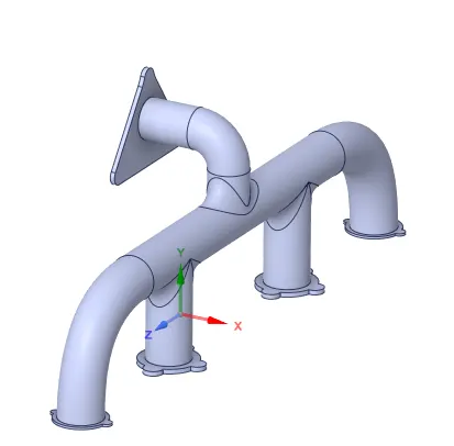
Below image is drag and drop in the spaceclaim from saved folder. The drag and drop option is alternative for importing geometry specially when the file format of geometry is not neutral. Geometry of exhaust port consist of for four inlets (exhaust gases collected form 4 different cylender) and one outlet (1 exhaust gas outlet).
Geometry Check
After importing model next step is to check for geometry error. If there exist some extra edges then remove them.
Volume Extraction
For flowing fluid volume extraction is done.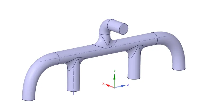
After Share Preparetion
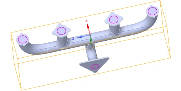
These two solid and fluid volume regions were combined using Share Topology feature.
Meshing
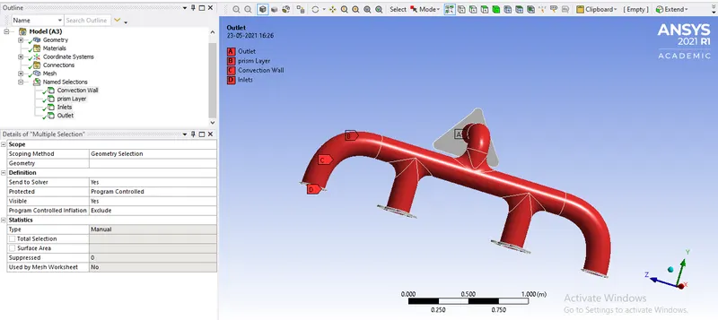
Before meshing the geometry we need to name the components as inlet, outlet, inner wall and HT wall.
To obtain more accurate results, the mesh is refined with added inflation layers. The heat transfer coefficient values can be accurately calculated at the surface between solid and fluid volumes with added inflation layers. For the solid volume, an element size of 0.0015 m is chosen to refine the mesh and for the fluid volume, an element size of 0.04 m is chosen to refine the mesh. Inflation layer is provided at the interface between solid and fluid with a total inflation thickness of 5 mm and growth rate of 1.2.
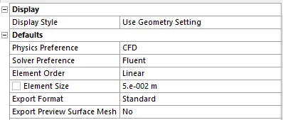
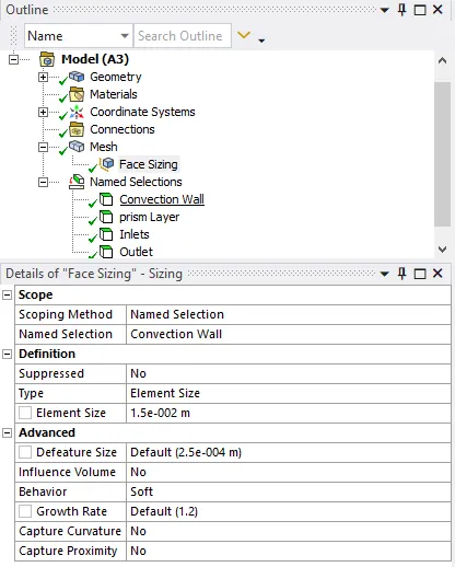

The mesh with inflation layers are as shown below:
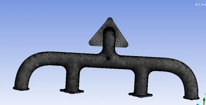
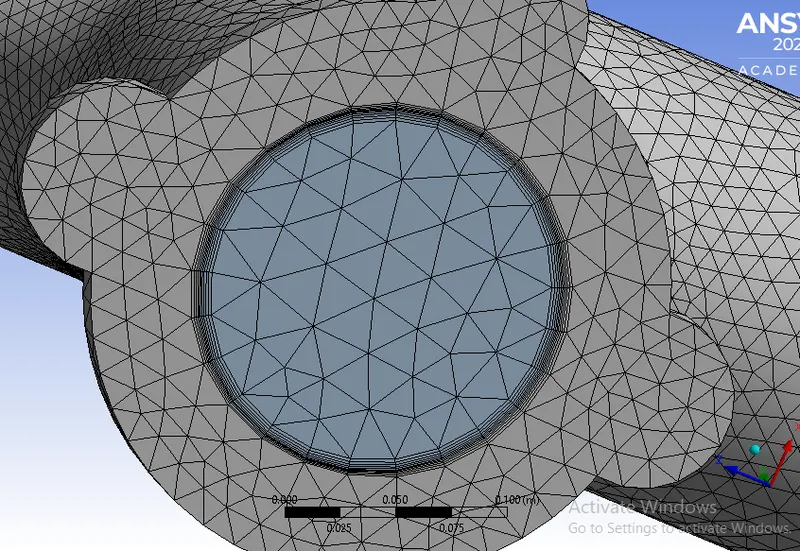
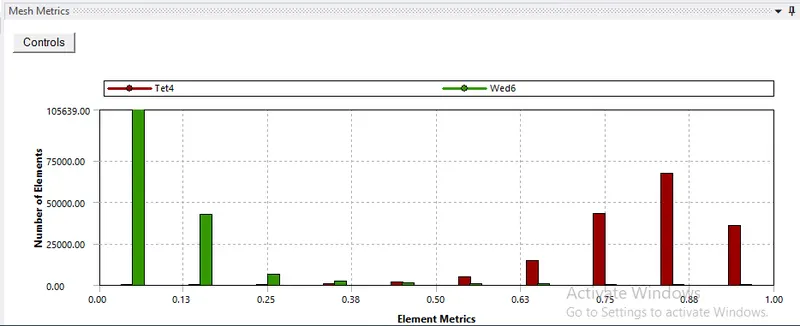
The element quality is optimum for subjecting mesh for simulation. It has a element size of 337774.

Solver Setting
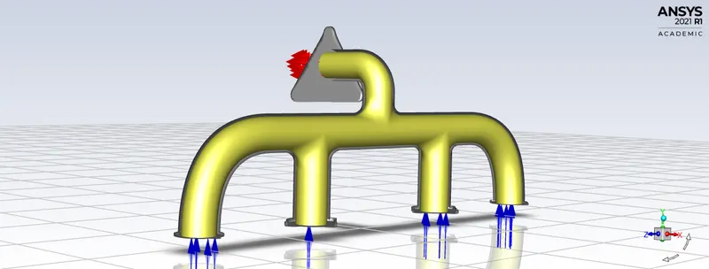
Simulation is done using double precision, Steady State Solver and checked for mesh and its quality.
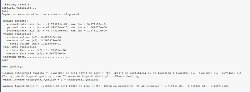
Energy equation is enabled as we are doing CHT simulation and standerd k-e model is used as turbulent model.
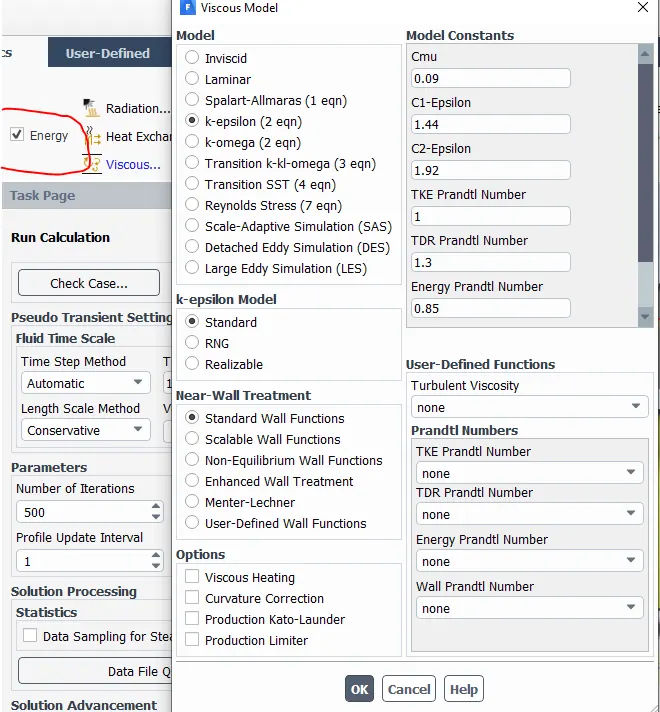
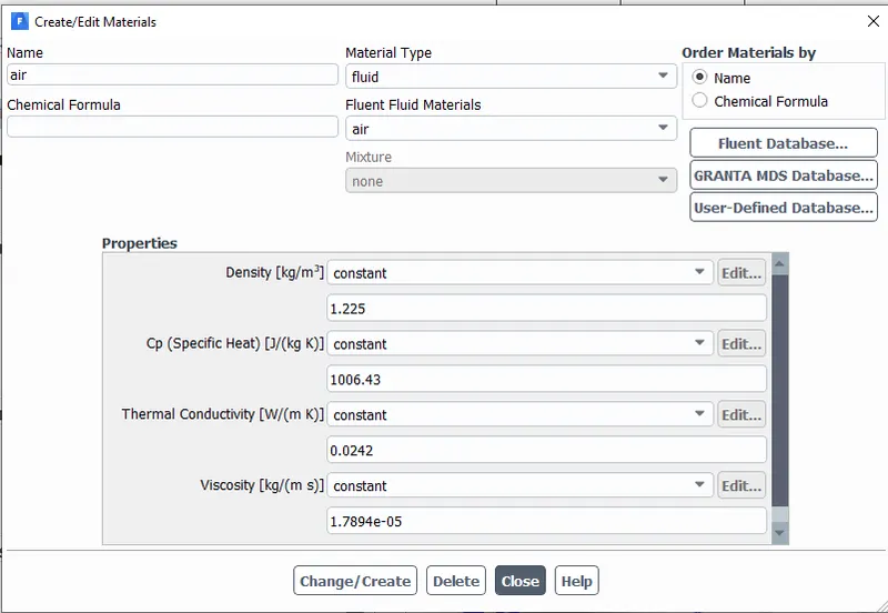
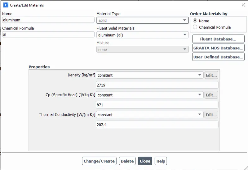
For solid volume the Alumium is taken as material and for fluid volume air is taken as material.
Boundary Conditions
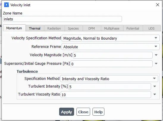
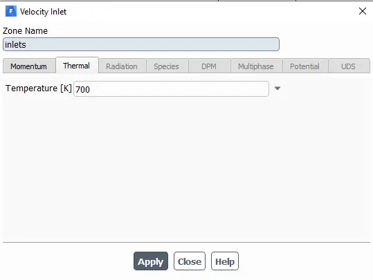
For Inlet Velocity b.c. is used with 5m/s velocity and 700K temperature and for outlet the pressure outlet is taken as b.c.
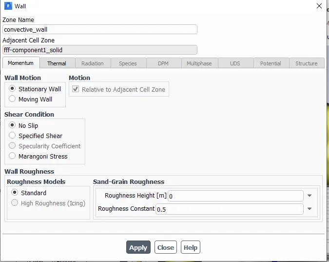
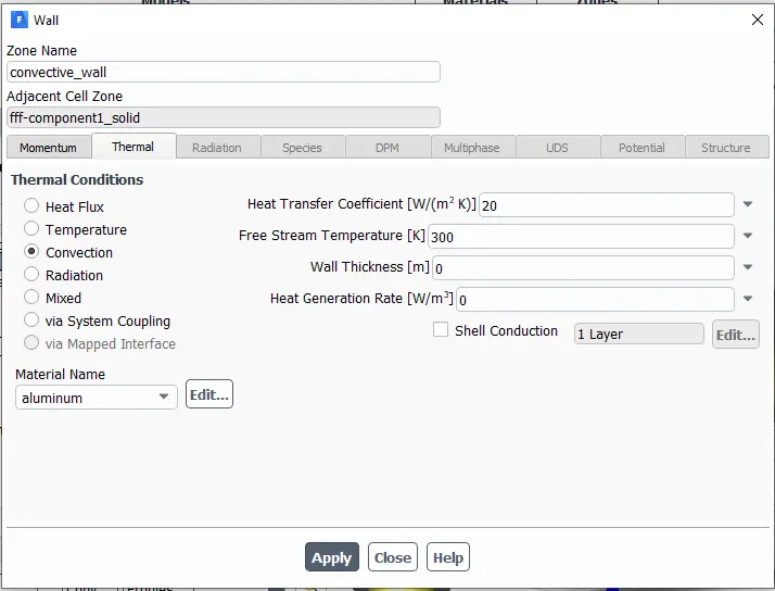
The outer wall is heat transfer wall therefore its thermal b.c. are set to convective stationary no slip wall with Heat Transfer Cofficint of 20`W/(m^2K)` with 300K free stream temperature.
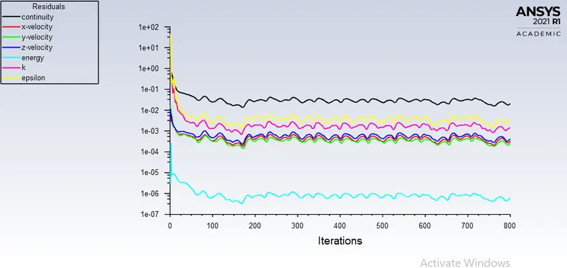
Residuals
Results
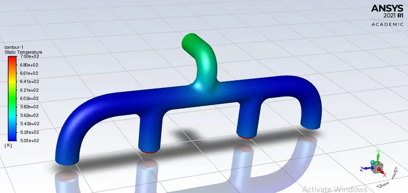
Temperature Contours
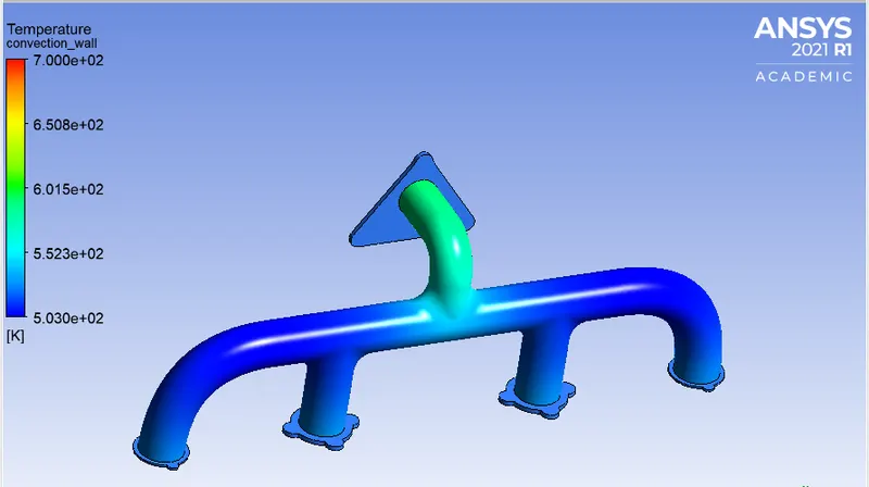
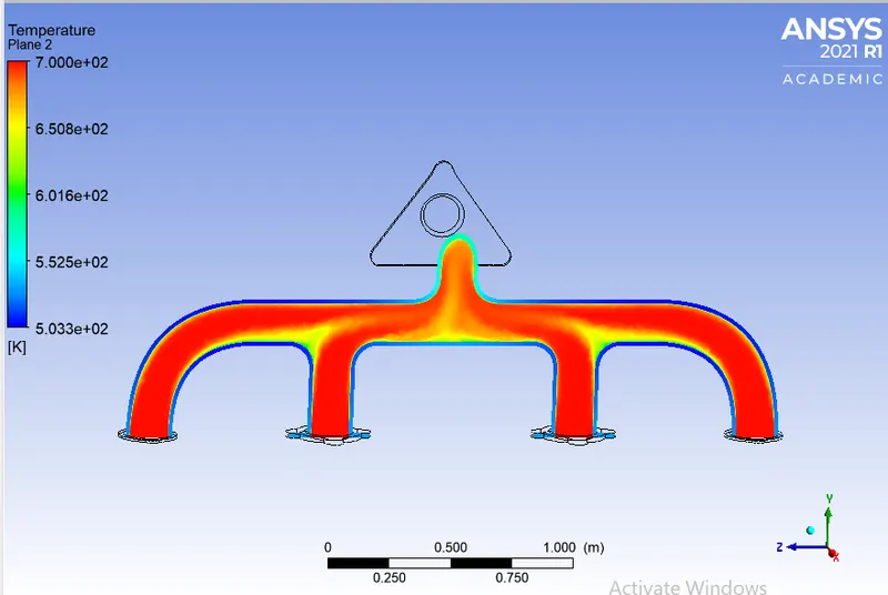
Temperature at outer wall is shown in the image below. It can be seen that the the temperature at the outer wall at the inlet is low as compared to that of at the outlet, this is because the velocity is lower at the inlets as compared to that at the outlet. So as the velocity increases, the Reynold's number increases, and the heat transfer coefficient also increases thus increasing the transfer of heat from the fluid to the solid.
Velocity streamline
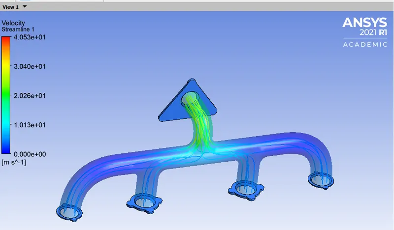
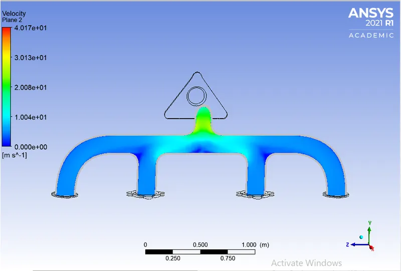
The Velocity streamline starting from the inlets is shown in the image below. Here we can see that the velocity is low in the inlet sections (the 4 inlets) whereas the velocity is higher at the outlet section, this is because of mass conservation. There are four inlets and only one outlet, all the faces are of same size i.e the area is same; and area times velocity is the flow rate.
A1V1 + A2V2 + A3V3 + A4V4 = A5V5
where, A1, A2,A3,A4 are the areas at inlet 1,2,3,4 respectively and A5 is the area at outlet
V1,V2,V3,V4 are the velocities at inlet 1,2,3,4 respectivelt and V5 is the velocity at outlet.
As A1=A2=A3=A4=A5,
Therefore
V1 + V2 + V3 + V4 = V5
Hence velocity at the outlet is higher than that at the inlets.
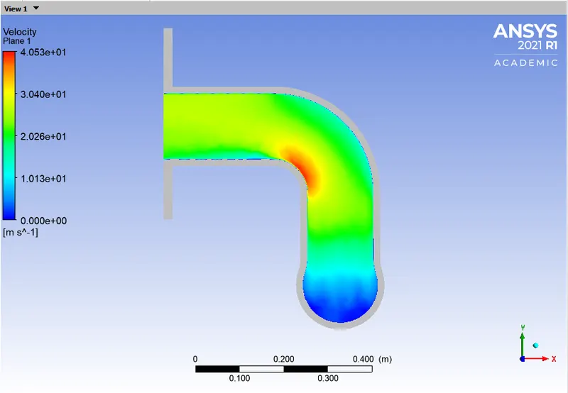
Using probes the velocity at the corner is found to be
Pressure Contours
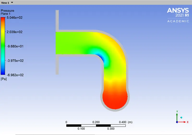
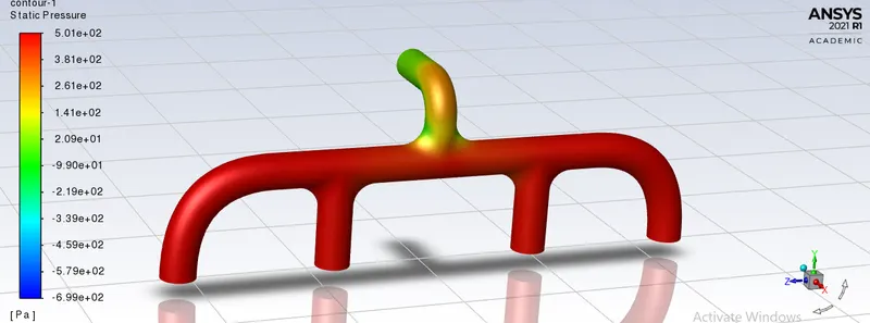
We can she at low velocity region pressure is high and viceversa.
Wall heat transfer coefficient and Y+ Value
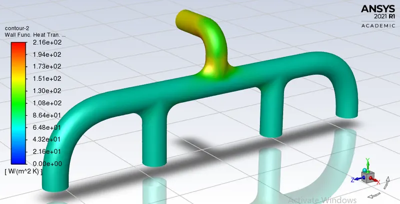
Wall heat transfer coefficient is a quantity that is calculated only at the wall that are adjacent to the fluid. With the inflation layers, notice that the wall heat transfer coefficient is captured accruately along the surface separating the solid and fluid volumes. Heat Transfer Cofficient is seen at very first cell of wall therefore as we used the y+ of 30(for k-e model)thus we can see the Heat Transfer coff. in between solid and fluid boundary. The maximum heat transfer coefficient is obtained at the same location where there is maximum velocity. The max. wall heat transfer cofficient is found to be 216 W/(m^2K)
3) How would you verify if the HTC predictions from the simulations are right? On what factors does the accuracy of the prediction depend on?
Nusselt's number is given by:-
`Nu=(h*L)/K`
therefore, `h= (Nu*K)/L`
where, h= Heat Transfer Coefficient
Nu= Nusselt's Number
K= Thermal conductivity coefficient
L= Characteristic Length
We know that the Nusselt's number is a function of Reynold's number, which in turn is a funtion of flow velocity
Therefore, HTC is directly proportional to flow velocity.
We can see from the images above that both the HTC and velocity are maximum near the outlet.
calculating theoretically:
So the value obtained by simulation is near to correct value. This error can be minimized by refining the mesh futher and choosing appropriate point for taking bulk temperature values. Hence, the HTC predictions from the simulations are correct.
Factors affecting the prediction are as follows:-
- Element Size and Quality - The finer the mesh, the accurate the results.
- Inflation Layer - It increases the quality of mesh near the boundary interface and helps to capture smooth plots of different quantities.
- Mesh at the solid-fluid interface - The mesh at the solid-fluid interface must be conformal.
Conclusion
- The velocity tends to increase from the inlet to the outlet because of mass conservation and mixing of air. hence, the high heat transfer coefficient at the junction is due to that high velocity and also when transfer of heat from fluid to solid is high.
- The internal flow velocity and its characteristics are affected by the Initial velocity, Pressure, the physical features of the geometry etc. that affect the heat transfer rates and hence CHT analysis is essential prior experimental analysis for better prediction life of the designed component.
- As shown in the plots, the hot exhaust gases passing through the manifold transfer some of the heat to it via convection. The amount of heat transfer can be related directly with the velocity of the exhaust. The temperature is lower where the flow is stagnate or is moving at the inlet velocity. As the velocity increases, so does the Reynolds number and hence the amount of heat transferred.
- Best methods to predict the accuacy of the result is by comparing the nusselt numbers from experiments and numerical results. The other method to verify is by comparing the results from published experimental results.
References
1) https://www.simscale.com/docs/content/simulation/analysis_types/OF_conjugateHeatTransfer.html
2) https://trivista.co.uk/design-and-analysis/cfd-overview/heat-transfer/