Week 4 - CHT Analysis on Exhaust port

CONJUGATE HEAT TRANSFER ANALYSIS ON EXHAUST PORT

PROBLEM STATEMENT:

1. Give a brief description of why and where a CHT analysis is used.
2. Maintain the y+ value according to the turbulence model and justify the results.
3. Calculate the wall/surface heat transfer coefficient on the internal solid surface & show the velocity & temperature contours in appropriate areas.
4. How would you verify if the HTC predictions from the simulations are right? On what factors does the accuracy of the prediction depend on?

AIM: The goal of this conjugate heat transfer analysis is to understand the heat transfer mechanisms between the fluid and metal in an exhaust port. The focus is on analyzing the heat transfer from the fluid to the metal. The objective is to study the distribution of temperature, velocity, and surface heat transfer coefficient over both the fluid and solid domains.

INTRODUCTION:

Conjugate heat transfer is a complex phenomenon that occurs in many industrial and natural systems. It involves the transfer of heat across multiple interfaces between different mediums, such as between a solid and a fluid, or between a fluid and a gas. The heat transfer occurs by a combination of conduction, convection, and radiation.

Conduction is the transfer of heat through a material by the movement of heat-carrying particles, such as atoms or molecules. In conjugate heat transfer, conduction occurs through the solid component, such as a wall or a heat exchanger.

Convection is the transfer of heat by the movement of a fluid or gas. In conjugate heat transfer, convection occurs in the fluid or gas component, such as a liquid or gas flowing over a solid wall. The fluid or gas carries heat from one location to another, and the heat is transferred to or from the solid surface.

Radiation is the transfer of heat by electromagnetic waves. In conjugate heat transfer, radiation occurs between the surfaces of the different mediums, such as between a solid surface and a fluid or gas.

Conjugate heat transfer is an important phenomenon in many industrial applications, such as power generation, chemical processing, and aerospace engineering. It is also important in natural systems, such as in the Earth's atmosphere and in the oceans. Understanding and modeling conjugate heat transfer is necessary for the design and optimization of these systems.

One of the challenges in conjugate heat transfer is that the different modes of heat transfer can interact with each other and affect the overall heat transfer rate. For example, the presence of a fluid flowing over a solid surface can change the heat transfer by conduction through the solid, and the heat transfer by convection in the fluid can be affected by the temperature of the solid surface. This makes the analysis and prediction of conjugate heat transfer a difficult task, requiring a combination of experimental and numerical methods.

PROCEDURE:

The simulation of this problem will be performed using ANSYS, a widely used commercially available CFD code. The CFD process will be carried out in several steps, including:

1. Geometry Creation/Pre Processing: The first step involves creating or cleaning up the geometry of the exhaust port for the analysis.

2. Meshing: The next step is to generate a mesh for the simulation. This involves dividing the geometry into small, manageable elements and defining the properties of these elements.

3. Solving: The third step involves solving the governing equations for the fluid flow and heat transfer. This is done using numerical methods and algorithms implemented in ANSYS.

4. Post-Processing: The final step involves analyzing the results of the simulation, including the distribution of temperature, velocity, and surface heat transfer coefficient. This information can be used to validate the simulation and make any necessary adjustments to the model.

This step-wise approach ensures that the simulation is accurate and reliable, and provides valuable information for optimizing the design of the exhaust port.

Geometry Creation/Pre Processing: Used a SOLIDWORKS PART FILE of exhaust port in Spaceclaim to perform pre-processing of CAD modelto be prepared to perform CFD simulation ready model.Performed the required necessary cleanup and the fluid volume is extracted from it. To share the information between two different domains Enabled the Share Topology option.

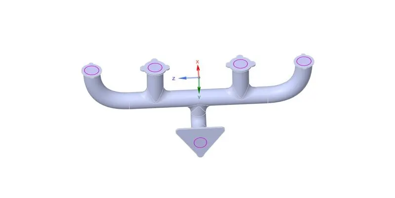
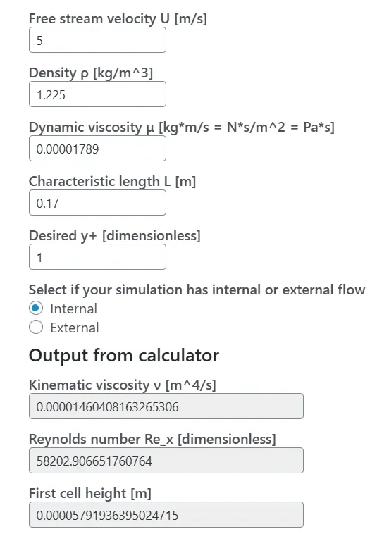
MESHING: Performed base line mesh on the exhaust port with 150mm length of the mesh elements. To capture more information on the boundaries and to capture the flow properly inserted Inflatin method at the interface of fluid and solid internal, by calculating the Y+value.

The Y+ value calculation was performed for a turbulent internal flow with a flow velocity of 5 m/sec and a characteristic length or diameter of the inlet cylinder of 0.17m. The calculation was based on the following parameters:

1. Flow velocity: 5 m/sec
2. Characteristic length or diameter of the inlet cylinder: 0.17m
3. First layer thickness: 0.06
4. Growth rate: 1.2%
5. Number of layers: 18.

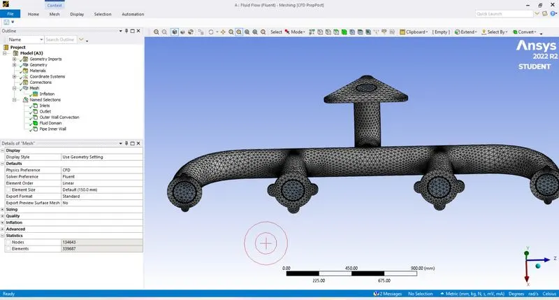
Mesh Elements Obtained are of 339687 elements. Nodes are of 134643.

SETUP:

General Settings:

Analysis type: Steady state

Solver: Pressure based solver

Method: COUPLED

Material Specifications:

For Fluid:

Material: Air

Density: 1.225 Kg/m³

Cp: 1006.43 J/(Kg K)

Thermal Conductivity: 0.0242 W/(m K)

Viscosity: 1.7894e-05 Kg/ (m-s)

For Solid:

Material: Aluminium

Density: 2719 Kg/m³

Cp: 871 J/(Kg K)

Thermal Conductivity: 202.4 W/(m K)

Viscous Model:

Model: K-Omega

K-Omega Model: SST (Shear Stress Transport) model

The SST model (Shear Stress Transport) is a turbulence model that combines the benefits of the k-epsilon and k-omega turbulence models. It's widely used for high Reynolds number flows with significant turbulence and complex flow physics. The SST model provides improved predictions of turbulence quantities, particularly in areas of the flow with strong adverse pressure gradients, and is well suited for problems involving separated flows and near-wall regions.

Boundary Conditions:

Inlet: Velocity-Inlet

Velocity:5m/sec

Outlet:Pressure-outlet

Gauge Total Pressure: 0 Pa

Initialization:

Hybrid Initialization

CASE1: 150mm BaseLine Mesh

Ran for 150 iterations.Following were the results.

SCALED RESIDUALS:

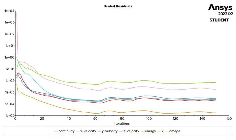
These results were not converged but it shows as the solution is stabilized.

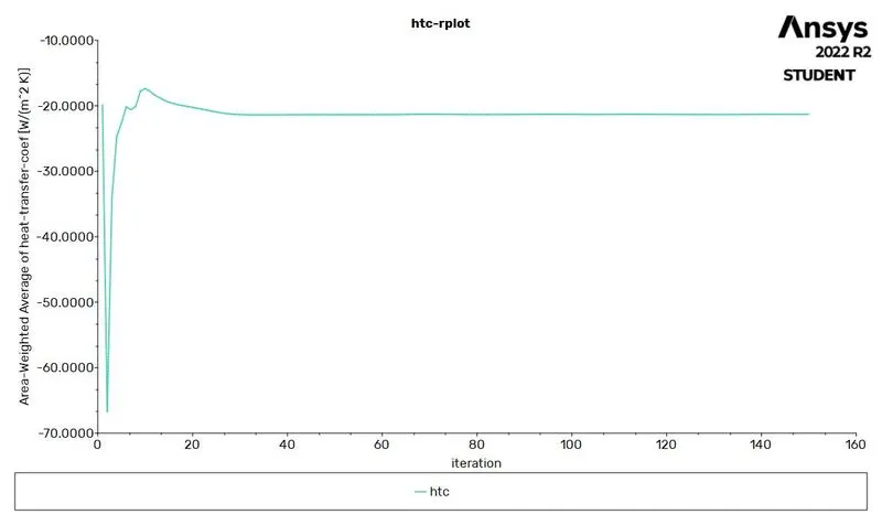
Above plot respresents the heat transfer coefficient from fluid to solid body, which seems like the solution the heat transfer is stabilized in less time.

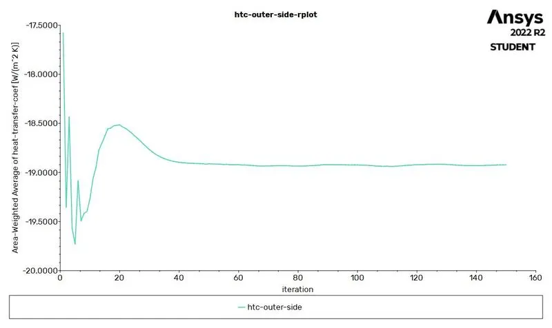
Heat transfer coefficient of outer wall is seems to be stabilized after 40 iterations.

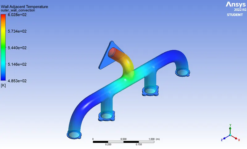
Streamline Plot:

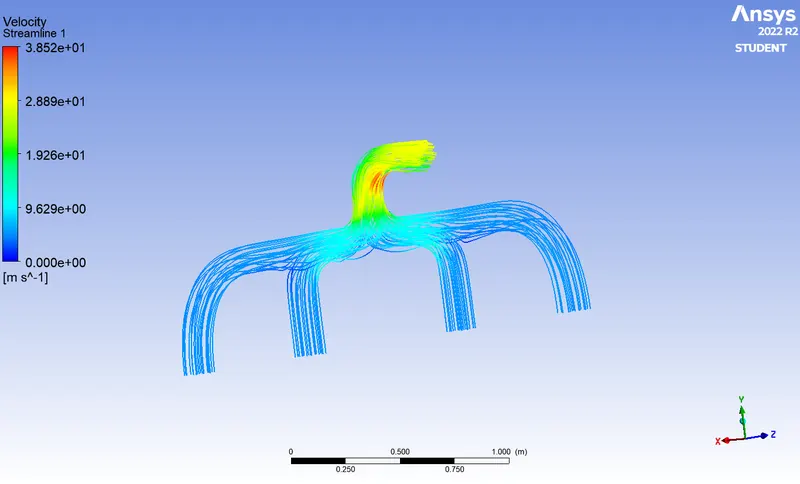
The plot provides a visual representation of the fluid flow pattern and helps in understanding the velocity and temperature distributions in different regions of the flow. It helps to identify any regions of high or low velocity or temperature and helps in identifying areas where further analysis may be required.

The above illustration depicts the velocity at the inlet and outlet, with red indicating the highest concentration of velocity. The color range represents the variations in velocity, with red indicating the maximum value and the other colors representing lower values.

Velocity Plot:

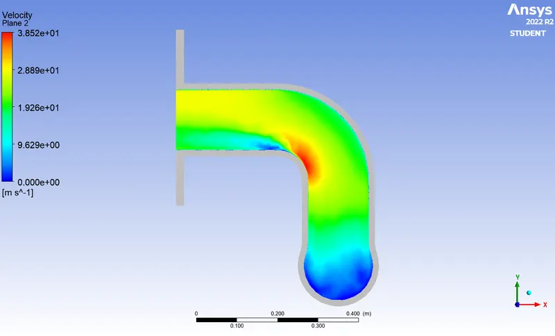
The above velocity plot demonstrates that there is a gradient in velocity at the exhaust port. If we increase the length of the port at the exhaust side, it will provide more space for the flow to mix, leading to a more uniform distribution of velocity, which is a critical factor for parameters such as temperature and pressure.

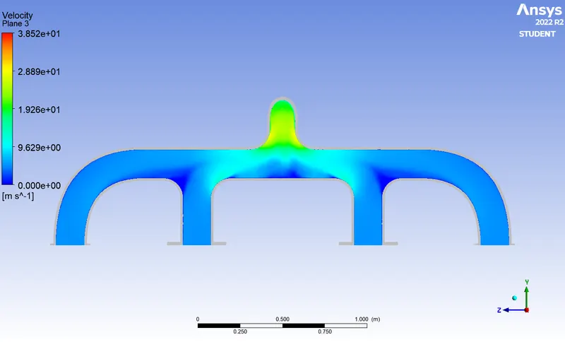
The velocity plots indicate that, due to the accumulation of mass flow from all four inlets into a single outlet, the velocity at the exhaust side section of the port is higher. We can see that flow is getting seperated bends of the pipe and gets mixed with the flow which will give us justification to use k-omega model for this problem where it can give better results for this type of flow.

Velocity vector plot

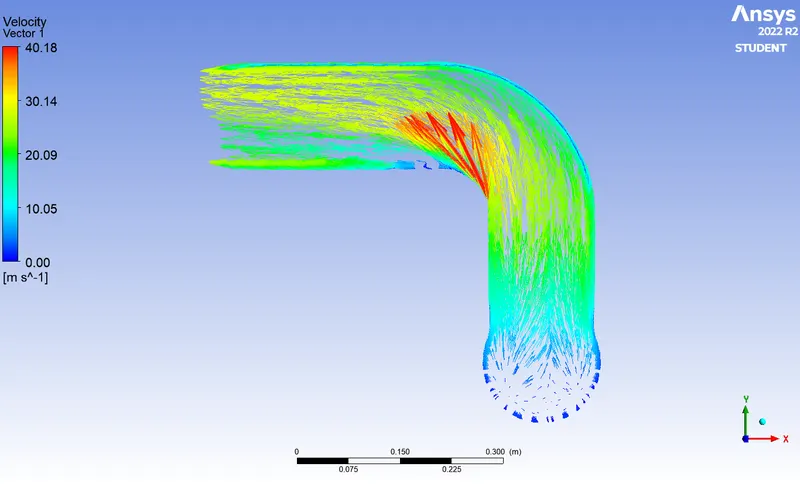
From the Vector Plot, it was observed that the flow separation occurred at the bend of the pipe, leading to an increase in the flow velocity. This resulted in a variation in temperature from the top to the bottom at the exhaust side of the port.

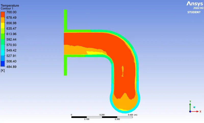
Temperature Plot

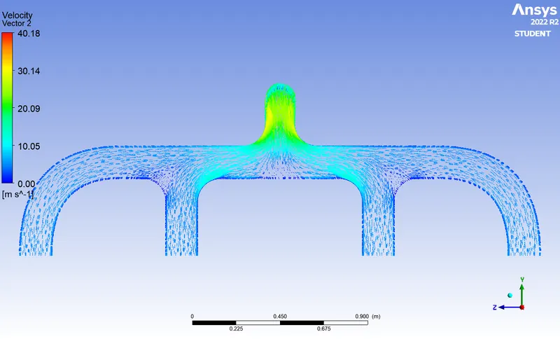
Velocity Vector Plot Outlet:

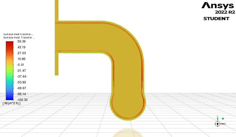
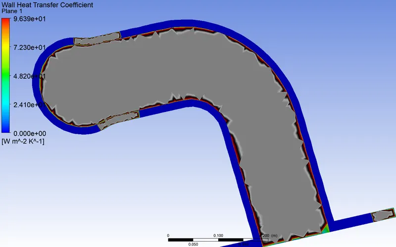
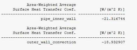
The above plot shows that the heat transfer is happening from fluid to the outer walls of the port at -21.3W/m^2 K.

Negative sign represents the heat being rejected.

VALIDATION:

To verify the accuracy of the HTC predictions from the simulations, it is necessary to compare them with experimental data or other validated simulations. Factors that affect the accuracy of the predictions include:

1. Model assumptions: The validity of the simulation results depends on the assumptions made in the turbulence, thermal and flow models used.

2. Grid resolution: The accuracy of the results depends on the quality and resolution of the computational grid used in the simulation.

3. Boundary conditions: The accuracy of the simulation results depends on the accuracy of the boundary conditions defined for the problem, such as fluid velocity, temperature, pressure, etc.

4. Physical properties of the fluid: The accuracy of the simulation results depends on the accuracy of the fluid properties such as viscosity, thermal conductivity, and specific heat used in the simulation.

5. Solution algorithm: The accuracy of the simulation results depends on the solution algorithm used in the simulation, such as finite volume method or finite element method.

By taking these factors into consideration and verifying the results with experimental data or other validated simulations, the accuracy of the HTC predictions can be improved.

Also with Nusselt number and its correlation calcultions we can compare the numerical calculation results with experimental results.

Reynolds Number for the flow is 58202.

The Nusselt number (Nu) is a dimensionless number used to describe the heat transfer rate through a fluid in relation to the heat transfer rate by conduction. It is defined as the ratio of convective heat transfer to conductive heat transfer and is expressed as:

Nu = hL/k

where h=convective heat transfer coefficient,

L =characteristic length,

k=Thermal conductivity of the fluid.

The Nusselt number can also be expressed as a function of the Reynolds number (Re) and the Prandtl number (Pr), as follows:

Nu = C Re^n Pr^m

where C, n, and m are constants that depend on the flow regime and the geometry of the system.

For Turbulent region Nusselt Number is,

Nusselt number(Nu)=0.0296(Re)^0.8*Pr^0.33

Prandtl Number

Prandtl number is defined as the ratio of momentum diffusivity (kinematic viscosity) to thermal diffusivity. It is a dimensionless quantity and represents the mixing of momentum and thermal energy in a fluid.

The Prandtl number for air is around 0.71.

Nusselt number(Nu)=0.0296(58202)^0.8*(0.71)^0.33 =171.3

Nusselt Number =171.3

From Simulation I got

h=21.3W/(m^2 K)

From Analytical the following are the results,

Nusselt number(Nu)=0.0296(58202)^0.8*(0.71)^0.33 =171.3

h=Nu*k/L

h=24.3W/(m^2 K)

INFERENCE:

From the above results we can see that the Analytical value is higher compared to the Simulated results. The simulation is getting a nearby results. By improving the meshing we may get better results.

CONCLUSION:

The simulation and validation of the internal flow through the exhaust port model showed that more heat transfer coefficient results in more heat energy transfer. Lower ambient conditions lead to higher heat transfer and a more efficient forced cooling system increases the velocity, which in turn increases the heat transfer coefficient and leads to better cooling. The design of the system should be proper for a uniform flow of fluid and to avoid flow separation. Additionally, the result was validated both analytically and using CFD. The computed average wall heat transfer coefficient by CFD and analytically were found to be similar. The use of CHT (conjugate heat transfer analysis) was also explained and found to be a useful study for the cooling system.

REFERENCES:

Book: Heat And Mass Transfer Fundamentals And Its Applications by YUNUS A CENGEL & AFSHIN A GAJAR

https://www.researchgate.net/publication/327775953_Modeling_of_Conjugate_Heat_Transfer

Heat And Mass Transfer Data Book.