Week 4 - CHT Analysis on Exhaust port

Aim: To perform a conjugate heat transfer analysis on an Exhaust port using ANSYS

Introduction:

Conjugate Heat Transfer (CHT):

Conjugate heat transfer is a type of heat transfer analysis between solids and fluids. This type of heat transfer includes both convection and conductive heat transfer, as well as both forced and natural convection.

This type of Analysis is majorly essential to find the Thermal simulations of heat exchangers, electronics, industrial machinery, battery simulation

What is Y+

y+ is a non-dimensional distance. It is often used to describe how coarse or fine a mesh is for a particular flow pattern. It is vital in turbulence modeling to determine the proper size of the cells near domain walls. The turbulence model wall laws restrict the y+ value at the wall. For instance, the standard K-epsilon model requires a wall y+ value between approximately 300 and 100. A faster flow near the wall will produce higher values of y+, so the grid size near the border must be reduced.

Solving and modeling approach

1. To solve the CHT, we initially create a fluid volume and inflations to the fluid for better results
2. we maintain the y+ value equal to 1, so we go with the k-omega model to solve the problem

Pre-processing and solver

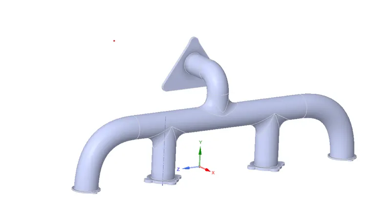
1. As it is an internal as well as external problem, we use the extract volume option to create a fluid body

Extract volume à select edges àclick right tick

2. Then use the share topology option for differentiating the fluid and wall or solid body in solving

Meshing

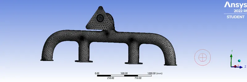
1. generate mesh by name selection, for individual meshing.

Insert mesh à external pipe as geometry with name selection option

2. For the internal wall of the fluid domain selected by faces

Insert à select faces

3. For fluid volume

Insert à select domain as the body

4. Insert inflation for fluid volume

By inserting inflationàselect fluid volume

5. Give parameters as 1^st layer thickness of 0.06, no of layers as 17, and growth rate of 1.3 (as calculated from y+ calculator)
6. Total elements of 495095

Set up and solving

1. Pressure based steady state solution
2. In physics, enable energy. As we also deal with heat transfer (energy interaction)
3. In cell, zone give the reference as fluid
4. Define the material, by default it takes air as fluid and aluminum as solid.
5. Give boundary conditions
6. Inlet = 5m/s, with input temperature 700K
7. Outlet = 0 vacuum pressure, and 300K temperature outlet
8. Ambient temperature or wall temperatures as 300K
9. The external pipe gives convective heat transfer coefficient as 20 w/m2K and temperature as 300K
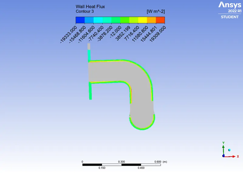
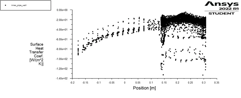
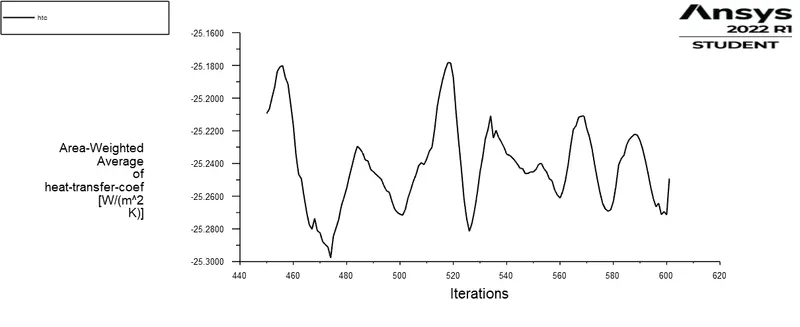
10. Define report, as we are analyzing the HTC, select surface report à average weighted area à wall flux à surface heat transfer coefficient à inner pipe wall
11. Initialize the setup à hybrid setup
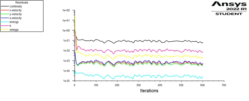
12. Then iterate until it gets converged.
13. Now compute the results, SHTC = inlet pipe wall = 25.3 W/m²
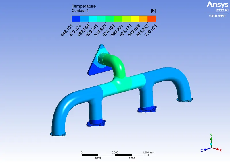
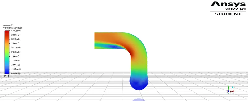
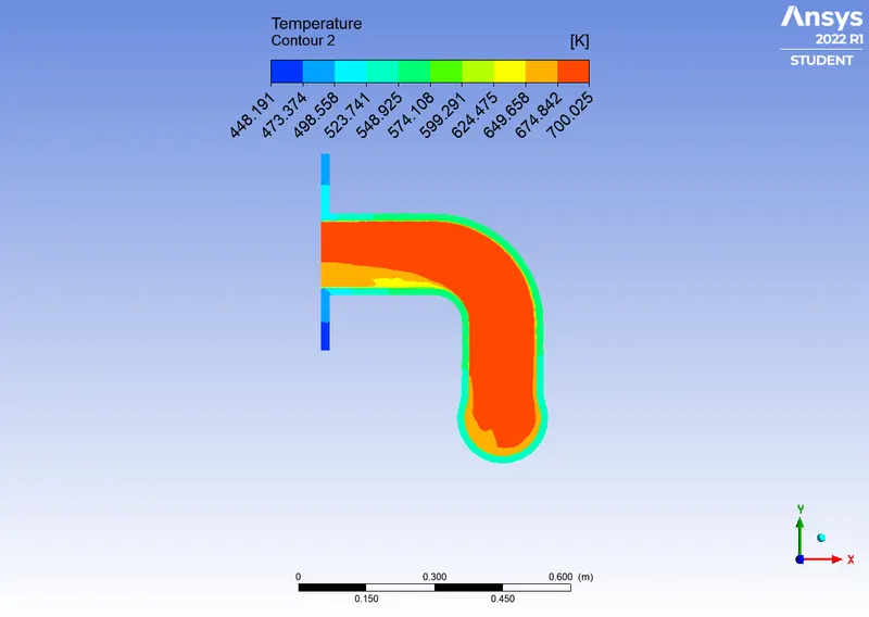
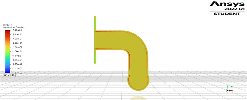
14. Define the contour plots of temperature, velocities, and SHTC plots at the central plane and in the body
15. We can also export the results to CFD post by selecting the Export option in the file.

Results

The contour of velocity, temperature, and surface heat transfer coefficients

Validation

For turbulent flow

Nusselt number is given as Nu=0.023*Re^(4/5)*Prⁿà equation 1

Where, n=0.4 (heating)

n=0.3 (cooling)

Nusselt number is a dimensional less number which is a ratio of convective heat transfer to the conductive heat transfer across the boundary

Nu=hL/K àequation 2

Where h= convective heat transfer coefficient

L= characteristic length

K= conductive heat transfer of fluid

Prandtl number = ratio of momentum diffusivity to thermal diffusivity

Pr=µCp/K = 0.743

Where µ=dynamic viscosity

Cp= specific heat capacity

K=conductive heat transfer coefficient of liquid

Reynolds number is a ratio of inertia force to the viscous force

Re=ρ*V*D/µ=56.353.6

Where, ρ= density of fluid

D=characteristic length

V= velocity of the fluid

µ=dynamic viscosity

From equation 1 and 2

hL/K=0.023*(Re)^4/5*Pr^0.3

h*.17/0.0242=0.023*(56353.6)^4/5*(0.743)^0.3

h=18.934 W/m²-k

Conclusion

1. Near-wall heat transfer coefficients are computed by maintaining y+ =1.
2. There is some variation in SHT computed (25.3) and Analytical (18.9), this could be because of the grid size.
3. finer mesh might give more accurate results, as the student version has a limit of 500000 elements.