Week 4 - CHT Analysis on Exhaust port

Aim – To simulate Conjugate Heat Transfer Analysis on exhaust port using Ansys Fluent.

Objective –

1. Brief description of where and why CHT analysis is used?
2. Justify results by maintaining the appropriate y+ value for the turbulence model.
3. Calculate Wall HTC and Surface HTC on the inner and on the surface of solid part exhaust ports?
4. Show Velocity and temperature contours in appropriate areas respectively.
5. Justify, how do verify if HTC predicted from simulations are right?
6. On what factors does the accuracy of the prediction depends?

Theory -

Conjugate heat transfer (CHT)

Conjugate heat transfer corresponds with the combination of heat transfer in solids fluids.

Heat Transfer in a Solid

In most cases, heat transfer in solids, if only due to conduction, is described by Fourier’s law defining the conductive heat flux, q, proportional to the temperature gradient.

For a time-dependent problem, the temperature field in an immobile solid verifies the following form of the heat equation:

Heat Transfer in a Fluid

Due to the fluid motion, three contributions to the heat equation are included:

1. The transport of fluid implies energy transport too, which appears in the heat equation as the convective contribution. Depending on the thermal properties of the fluid and the flow regime, either the convective or the conductive heat transfer can dominate.
2. The viscous effects of the fluid flow produce fluid heating. This term is often neglected, nevertheless, its contribution is noticeable to fast flow in viscous fluids.
3. As soon as a fluid density is temperature-dependent, a pressure work term contributes to the heat equation. This accounts for the well-known effect that, for example, compressing air produces heat.

Accounting for these contributions, in addition to conduction, results in the following transient heat equation for the temperature field in a fluid:

Conjugate Heat Transfer Applications

• Internal combustion engine

• Cross Flow heat temperature,
• Integrated Circuit Chips,

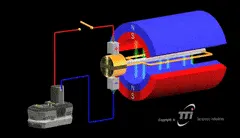
• HVAC
• turbocharger,
• Cooling of Electronic Devices, Burners, and Combuster
• Heat transfer in fin arrays, micro-channels, and ribbed passages.
• Drying of a porous flat plate.

Why CHT analysis?

• Conjugate heat transfer (CHT) analysis can accurately predict heat transfer by simultaneous solving all the relevant solid and fluid flow field heat transfer processes, for example, conduction through solids, free and forced convection in the gases/fluids, and thermal radiation.
• The CHT approach has an advantage over FEA thermal analysis.
• In that wall heat transfer coefficients and their local variations on surfaces are directly calculated within the model rather than based on simplified empirical calculations.
• The CHT approach, therefore, has benefits for those applications where heat transfer is either non-uniform or difficult to calculate empirically.

Wall Heat Transfer Coefficient and Y+ value –

1. Wall HTC is the quantity that can be calculated at the first cell layer of the wall adjacent to that of fluid.
2. With the inflation layer, the user can notice accurate capturing of Wall HTC along the surface separating solid and fluid volumes.
3. Maximum HTC is predicted/captured at the same location of maximum velocity.
4. In the k-omega turbulence model which is to be used in this case the desired y+ plus value is 1-10

Analytical solution

As the working fluid for CHT analysis is air so density ρ = 1.225, viscosity μ = 1.7894e−05, the characteristic length for the internal flow of the pipe is its mean diameter L = 0.17m, and the velocity of the inlet air is v = 5m/s

So reynolds number R = (ρ*v*L)/μ = 58189.8960

The Reynolds number for the given flow is 58189.8960 which suggests that the flow is turbulent, the Dittus Bolter heat transfer coefficient relation can be used to determine the Nusselt number which is described mathematically as follows

Nu = 0.023*(Re^(4/5))*(Pr^0.3)

Pr = μ*Cp/k

Thermal conductivity of air k = 0.024 W/mK

Specific heat at constant pressure Cp = 1075 J/kgK

so Pr = 0.8015

so Nu = 139.5651

and as Nu = h*L/k

so convective heat transfer coefficient h = Nu*k/L = 19.7033 W/(m^2)K

Modeling approach

For this CHT case study, two models are created with the k-omega turbulence model one with the mesh element size of 50mm and the other with the mesh element size of 10mm, and the results obtained will be compared with the calculated analytical solution and the optimized mesh element size will be decided from the obtained results which conforms more with the analytical solution.

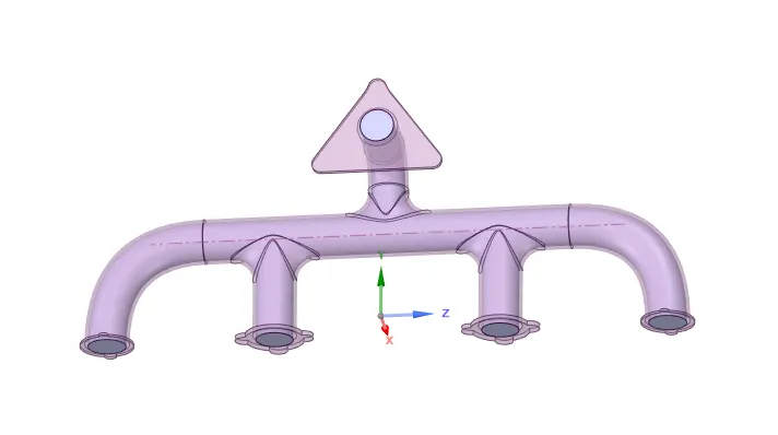
Given model is imported to the SpaceClaim work area and the volume of the exhaust pipe is extracted as shown in the figure below

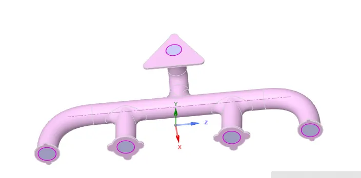
And then the boundaries between the extracted volume and the exhaust pipe walls are shared for generating common node points while meshing

Case 1:

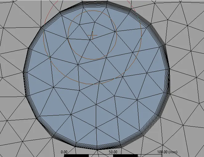
The baseline mesh with a mesh element size of 50mm is generated for both exhaust pipe and volume

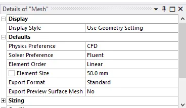
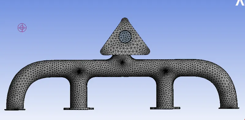
all the surfaces of the volume and exhaust pipes are named as shown in the figure below

for the inflation first layer thickness with desired Yplus value of 10 the Yplus calculator is used and the first layer thickness is calculated as 0.5mm

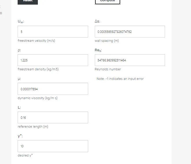
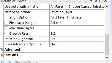
And in the setup pressure-based steady state solver is used with the k-omega SST turbulence model

The inlet fluid material is air and the material of the pipe wall is Aluminium with a convective heat transfer coefficient of 20 W/m^2K

and the inlet air is supplied at the velocity of 5m/s and at a temperature of 700k

To calculate the heat transfer coefficient at the inner wall of the exhaust pipe a heat transfer coefficient definition is created and the results are as shown in the figure below

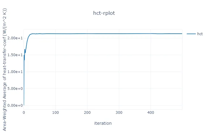
from the plot, it can be seen that the desired result was converger so the iteration was limited to 500 even if the solution was not converged

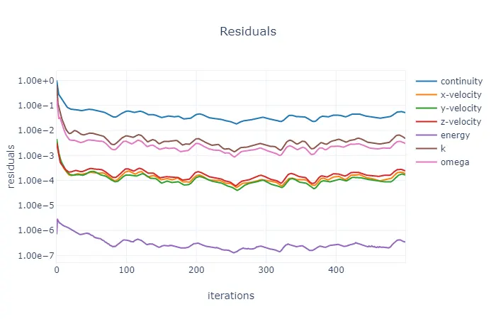
Residuals:

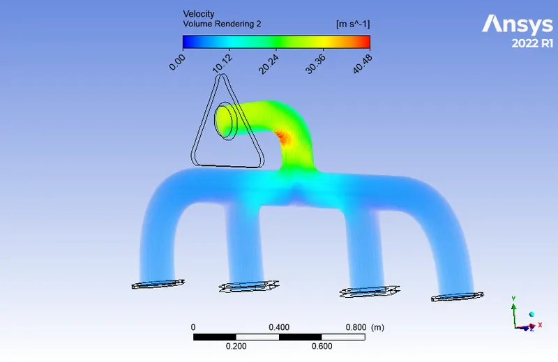
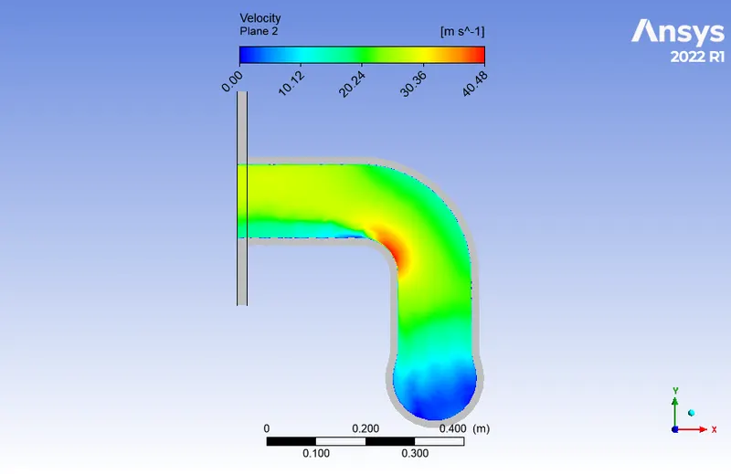
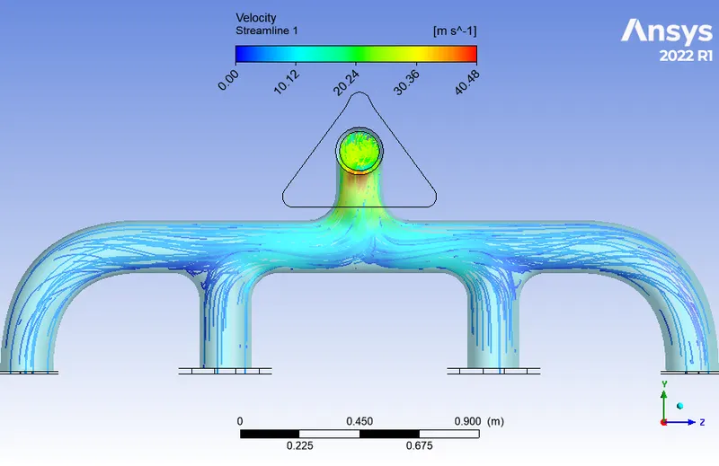
Velocity contour and streamline:

Temperature Contour:

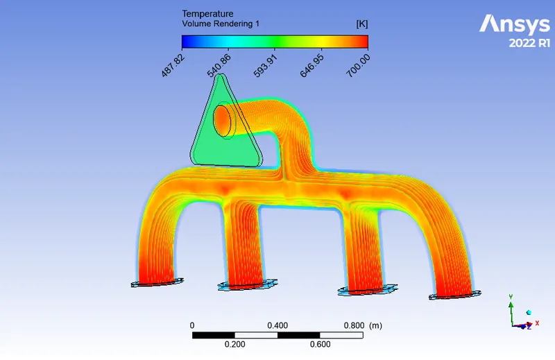
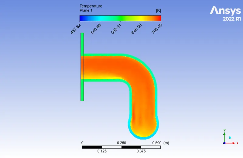
Surface heat transfer coefficient contour:

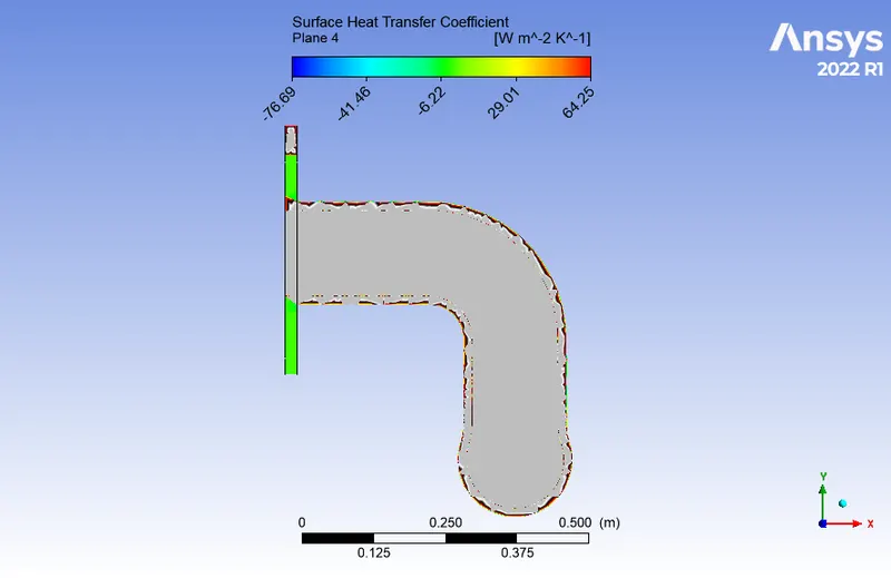
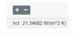
From the results and contours, it can be concluded that the velocity is high at the inlet and the surface heat transfer coefficient varies slightly from the analytical resluts.

Case 2:

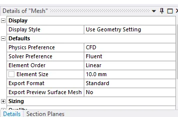
The baseline mesh with a mesh element size of 25mm is generated for both exhaust pipe and volume

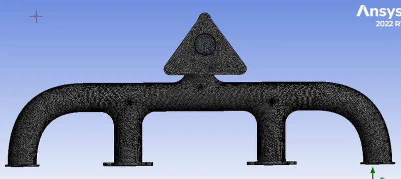
all the surfaces of the volume and exhaust pipes are named as shown in the figure below

for the inflation first layer thickness with desired Yplus value of 10 the Yplus calculator is used and the first layer thickness is calculated as 0.5mm

And in the setup pressure-based steady state solver is used with the k-omega SST turbulence model

The inlet fluid material is air and the material of the pipe wall is Aluminium with a convective heat transfer coefficient of 20 W/m^2K

and the inlet air is supplied at the velocity of 5m/s and at a temperature of 700k

To calculate the heat transfer coefficient at the inner wall of the exhaust pipe a heat transfer coefficient definition is created and the results are as shown in the figure below

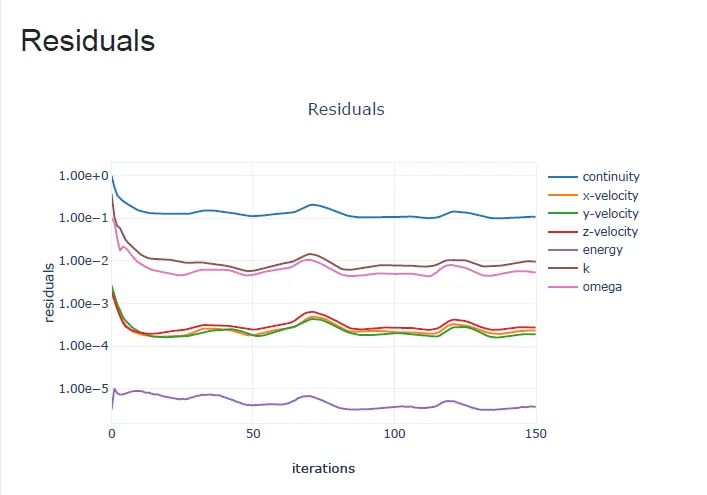
from the plot, it can be seen that the desired result was converger so the iteration was limited to 250 even if the solution was not converged

Residuals:

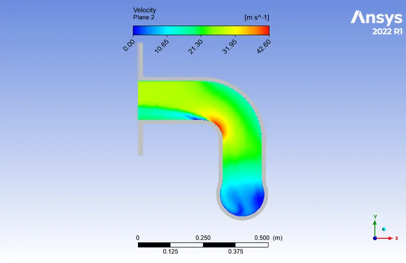
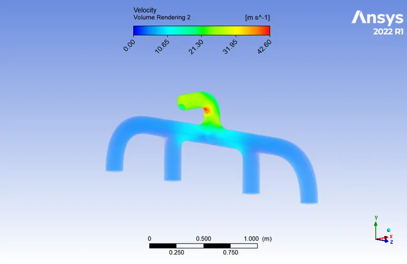
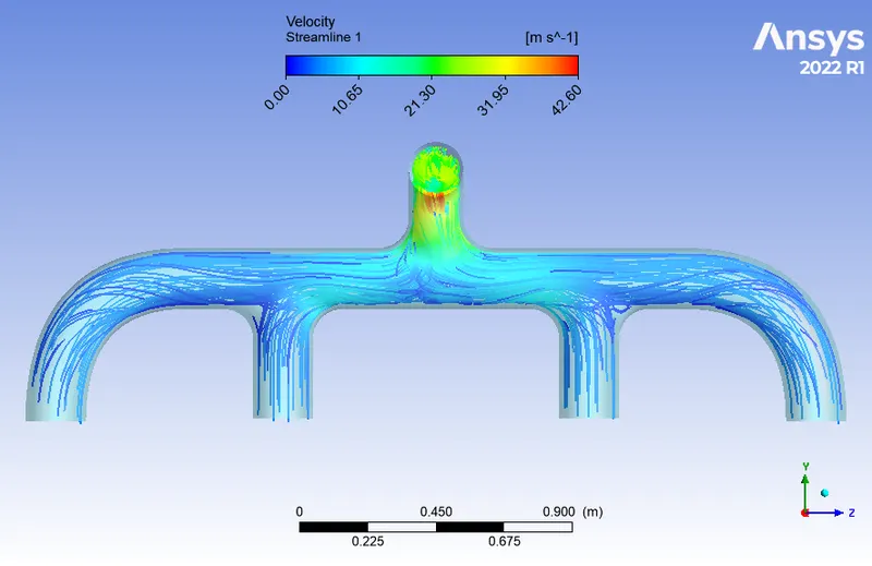
Velocity contour:

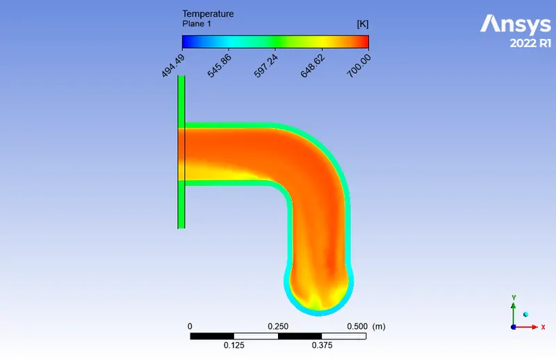
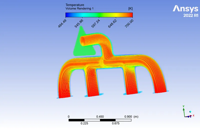
Temperature contour:

Surface Heat transfer coefficient contour:

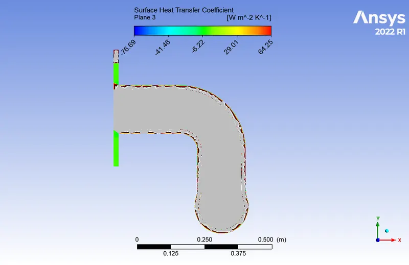
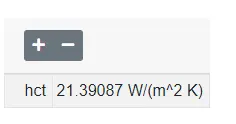
From the results and contours, it can be concluded that the velocity is high at the inlet and the surface heat transfer coefficient varies slightly from the analytical resluts. And also that there is no siginificant improvent in the accuracy of the results so the 50 mm mesh element size can be considered optimal.

Conclusion

• The CHT analysis on the exhaust port was simulated successfully on ANSYS-FLUENT.
• The pressure-based, coupled scheme solver is used to discretize the whole geometry.
• The analytical value of the heat transfer coefficient is
• The deviation of numerical heat transfer coefficient values from the analytical solution was found to be within 5% to 10% for the second and final mesh refinement are found to be in compliance with the industrial standards.
• The grid independence test was also observed during mesh refinement. The value of the heat transfer coefficient for the second and final mesh refinement are close to each other. It is important that we limit ourselves to the second refinement only to save the computational time and cost of the project.
  
• The value of the heat transfer coefficient is located in the cell adjacent to the wall which allows us to choose the value of Y+=1(viscous sublayer) and the turbulent model k−ω SST.
• The presence of the boundary layer is quite visible near the inlet of the pipe where the viscous force makes the velocity near the wall to be zero causing a no-slip condition to occur., but as the flow is turbulent in nature Reynolds number 58189.8960 the velocity profile goes from flat to the flutter and the boundary layer vanishes at the outlet.
• The velocity at the outlet is higher than the velocity at the inlet can be attributed to the presence of four inlets and one outlet.
• The accuracy of the heat transfer coefficient depends on selecting the suitable value of Y+ and turbulence model k−ω SST model. The heat transfer coefficient values predicted by CFD were validated against the numerical solution depicted the deviation in the range of 5% to 10% which is in compliance with industrial standards. However, the accuracy of k−ω SST model itself depends on the accuracy of the analytical solution, flow properties, and geometry. The values predicted by the baseline mesh and the refined mesh were close to each other this can be attributed to the fact that the boundary keeps on growing and declining from the inlet to the outlet owing to change in velocity, thus the value is predominant at the outlet section of the exhaust port.