Week 4 - CHT Analysis on Exhaust port

CHT Analysis on Exhaust port

Objective:

1. brief description of why and where a CHT analysis is used.
2. simulate both fluid flow and also the heat transfer to the solid i.e., CHT Analysis on an Exhaust port
3. calculate the wall heat transfer coefficient on the internal solid surface & show the velocity & temperature contours in appropriate areas.
4. verify the HTC predictions from the simulations are right? And mention the factors that the accuracy of the prediction depends on.

Conjugate Heat Transfer (CHT) analysis:

Conjugate Heat Transfer analysis allows for the simulation of heat transfer between solid and fluid domains by exchanging thermal energy at the interfaces between them and transported via conduction within solids and additionally via convection within fluid domains.

Conjugate heat transfer analysis can accurately predict heat transfer by simultaneous solving all the relevant solid and flow field heat transfer processes. Conjugate heat transfer corresponds with the combination of heat transfer in solids and heat transfer in fluids.

In solids, conduction often dominates whereas in fluids, convection usually dominates. Conjugate heat transfer is observed in many situations for example: conduction through solids, free and forced convection in the gases/fluids and thermal radiation.

The three main modes of heat transfer:

‐ Conduction is heat transfer that occurs when a temperature difference exists across a stationary medium.

‐ Convection is the heat transfer between a surface and a moving fluid when there is a temperature difference between the two.

‐ Radiation (thermal radiation) is the emission of energy in the form of electromagnetic waves. In the absence of an intervening medium ,there is net heat transfer by radiation between two surfaces at different temperatures.

Procedure

We will simulate both fluid flow and also the heat transfer to the solid i.e., CHT Analysis on an Exhaust port with the steady state .Then for solving we

follow the below procedure:

1)Geometry setup

2)Meshing

3) Problem setup

4)Solving

5)Post processing

Then we calculate the wall/surface heat transfer coefficient on the internal solid surface & show the velocity & temperature contours in appropriate areas.

Given model

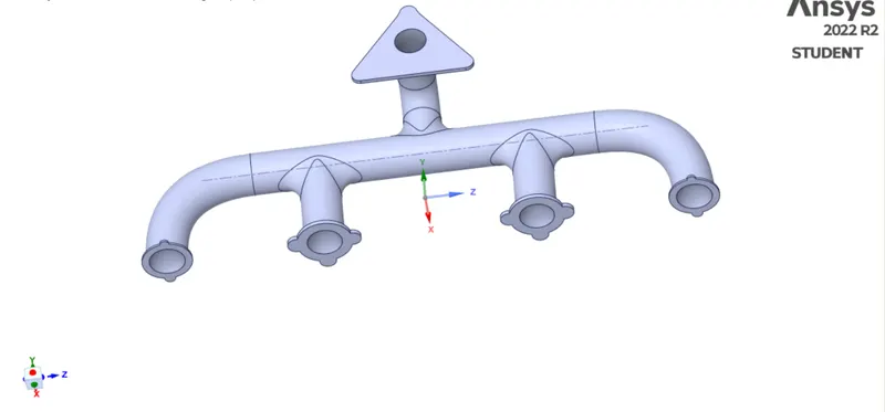
• Geometry setup

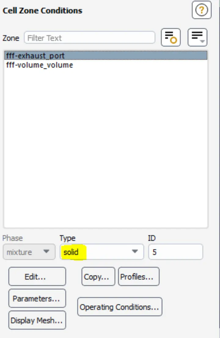
In fluent module we have to open space Claim and import the geometry. If you look closely at the geometry, it has solid part. So first let us extract the fluid volume.

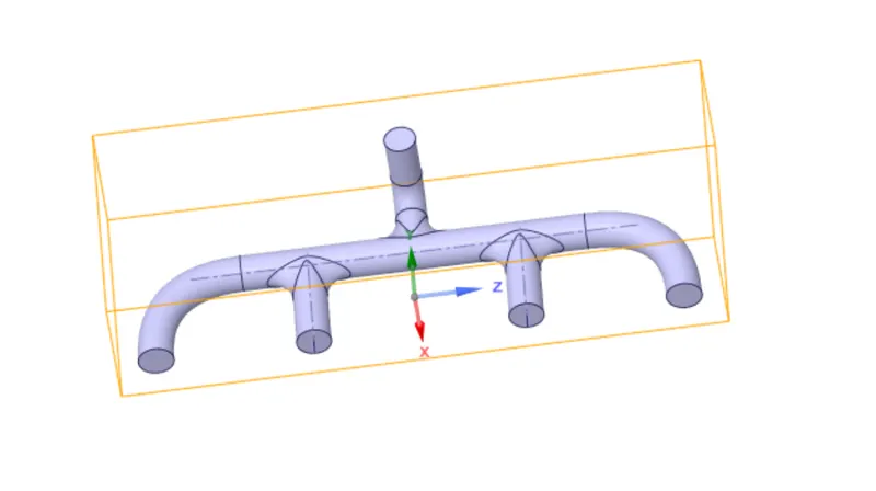
Click >>prepare >> volume extract >> select edge selection >> then select all the edges of inlet and outlet >> then click ok. Fluid volume will be created.

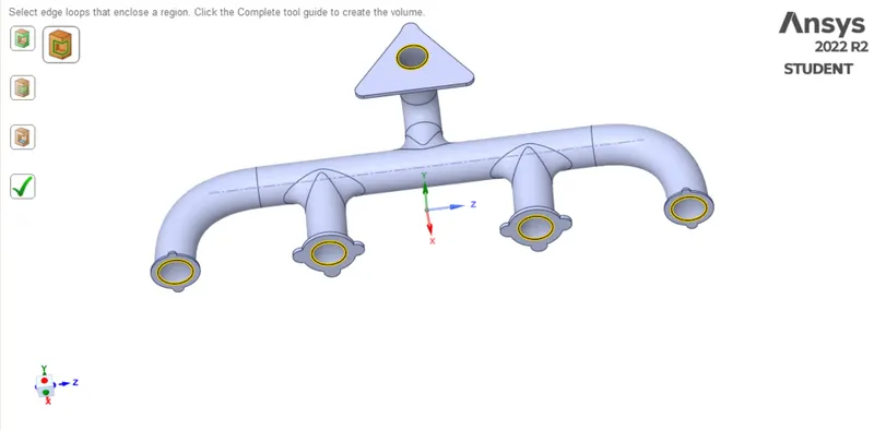
we need to share topology to create connections for inner surfaces. Without sharing topology, the mesh will be created in uneven node points(unconnected) which is nearby edges and faces.

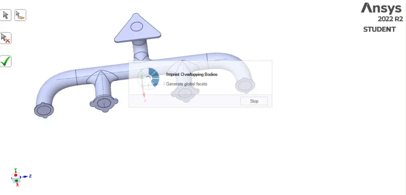
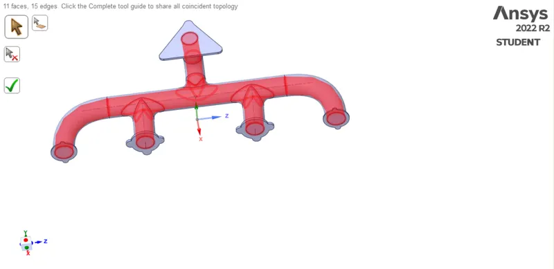
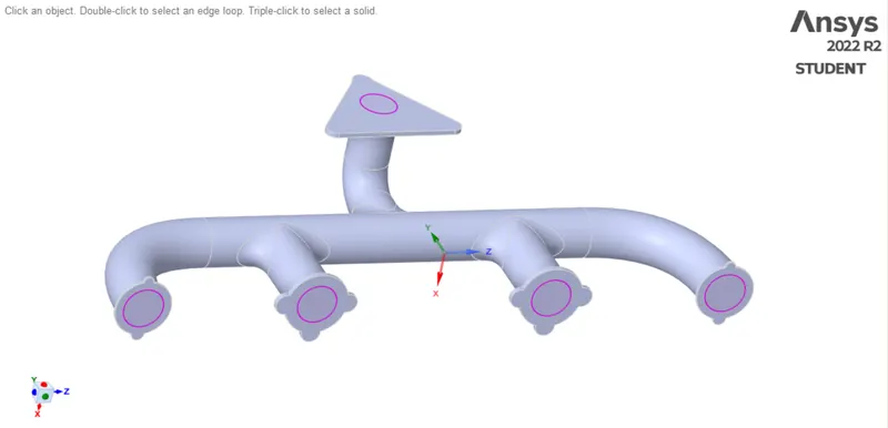
After this step the geometry part is completed, close the space Claim, the progress will be saved automatically.

• Meshing

After closing space claim, Right Click on the mesh and click edit.

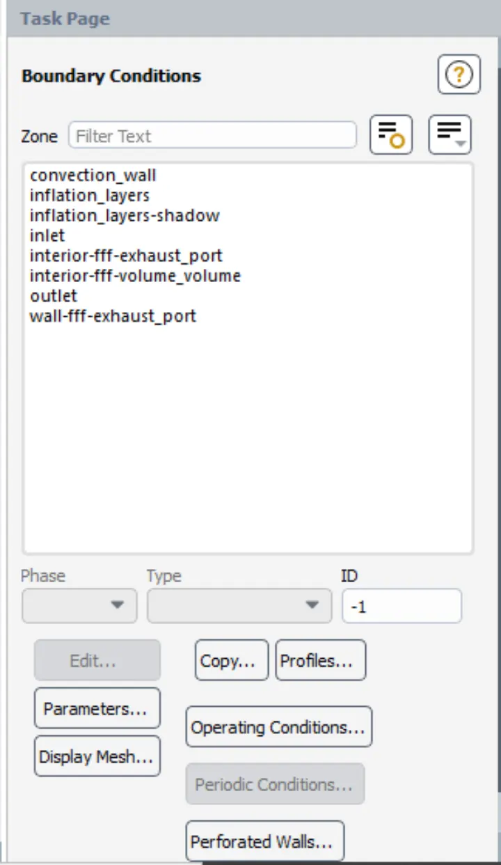
Creating name for model >>steps: select the edge you want to name by using edge selection >> then press N or right click and select create new name >> name the selection. In a similar way we name our inlets, outlet, and for outer wall just double click on the outer part anywhere and will automatically select the faces we require and we name it as convective wall.

Case1) 150mm

Click the mesh option in the side window, Right click on MESH option and click generate mesh. At first, we created the mesh on the default mesh size (150mm). Then for the edges we are creating an inflation layer for finer mesh so the flow is captured accurately.

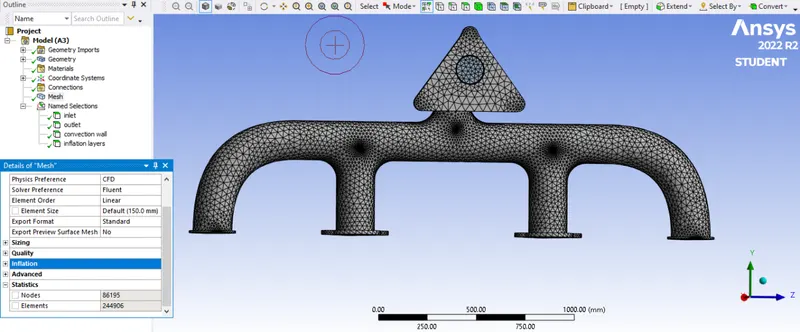
Inflation Layer

In this step, we create a first layer height of 0.5 mm thickness and growth rate of 1.2%, over and around the co-incident layer, to accurately capture the sharing of information between the solid and fluid surfaces. Here they created nodes (86195) and elements (244906).

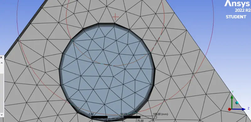
• Setup

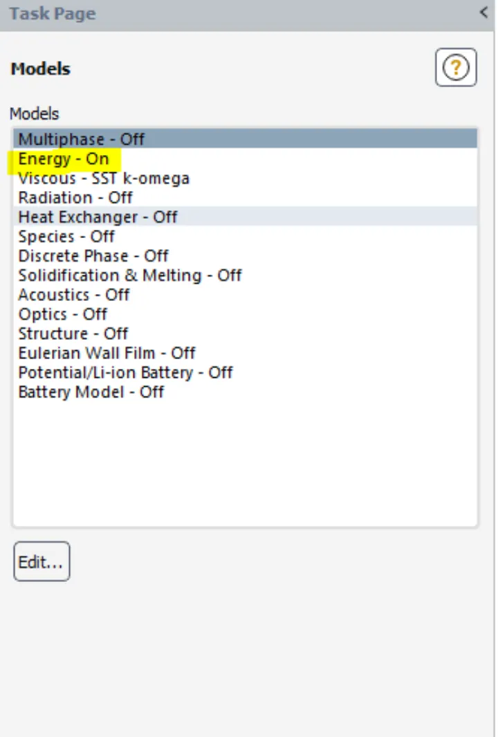
Right click on the setup and click edit select double precision and solver as 4 for better results. In this problem we use steady state solver. For heat transfer problems we need to enable energy equations.

Boundary conditions: We will basically give our boundary conditions here such as inlet velocity and outlet conditions.

we give,

Inlet velocity: 5 m/sec

temperature: 700K

In convection wall conditions select >>edit >>in thermal conditions select >> convection mode >>

Heat transfer Coefficient input as 20 W/(m²K) >> click Apply

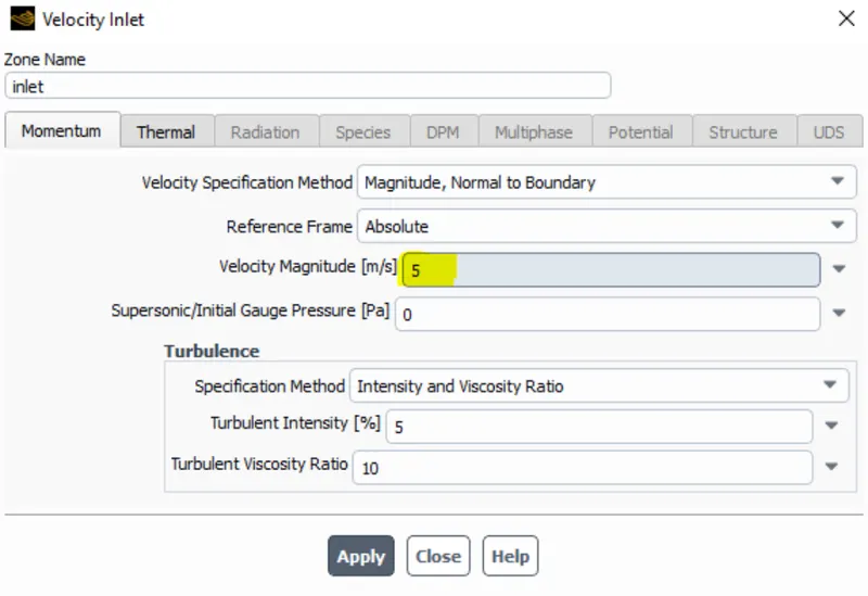
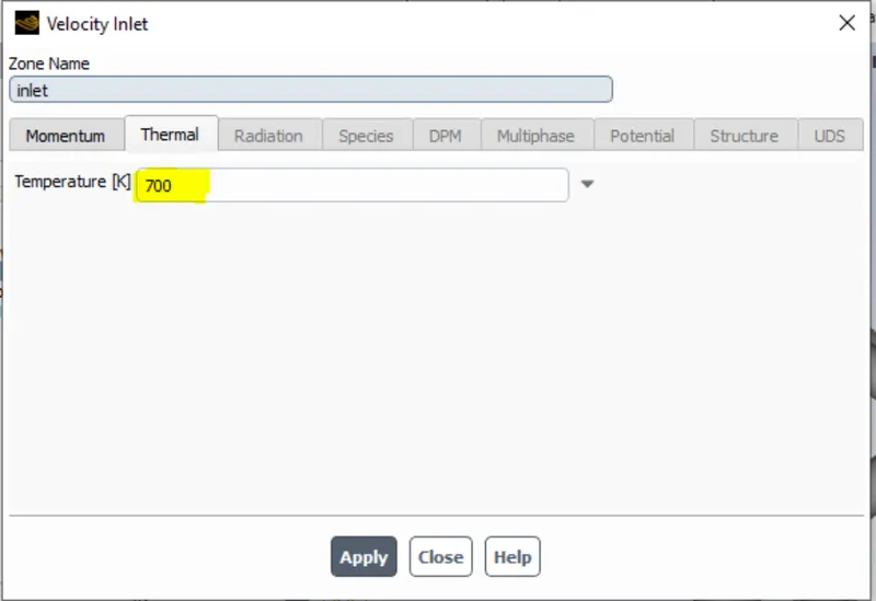
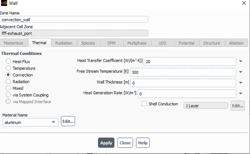
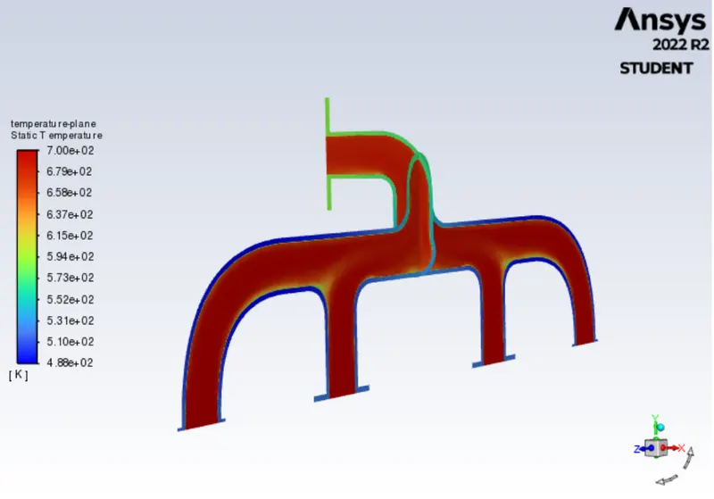
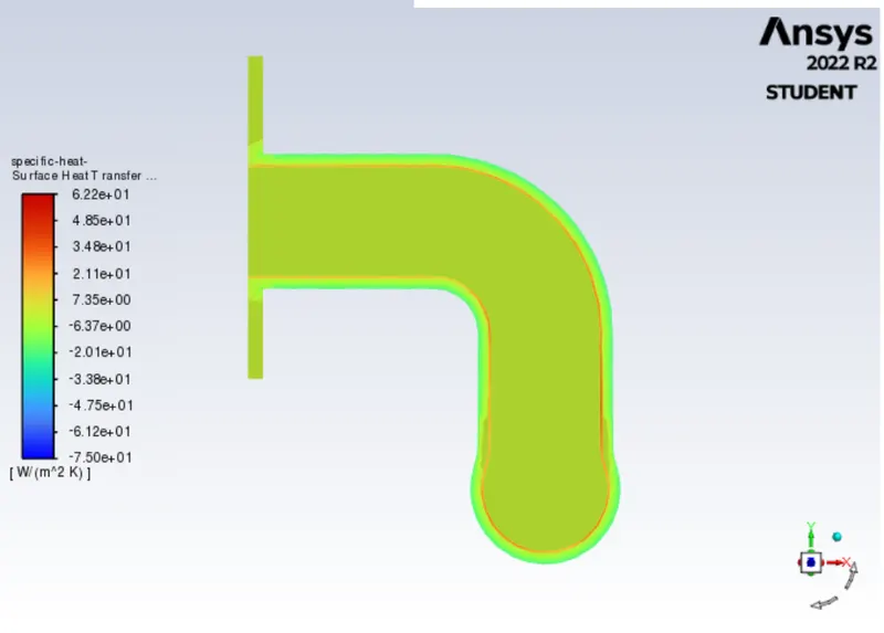
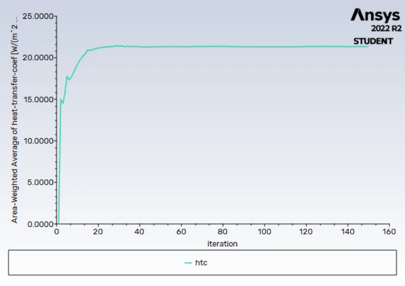
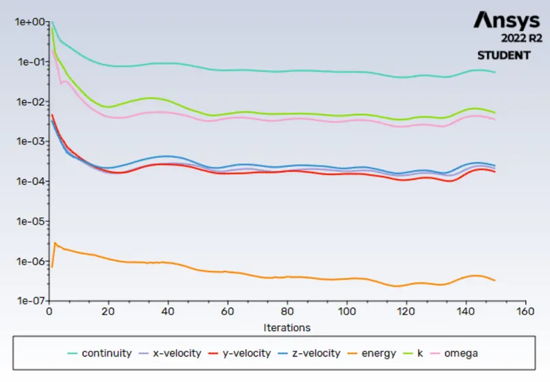
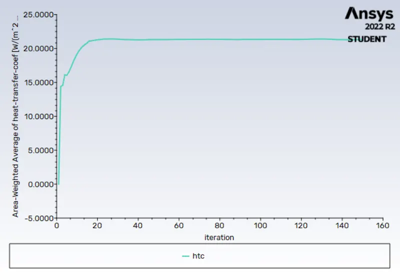
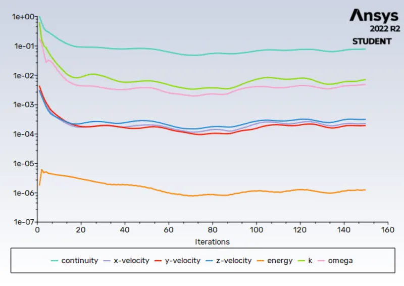
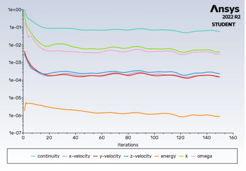
Now we are almost ready to run the simulation, but as the solution is being solved, we want to monitor different flow quantities while the solution is being generated. But before that we have to initialize the domain. We use the Hybrid initialization, this provides a initial condition. Click on run calculation for 150 iterations. Then we can see that in the residual plot that residuals drop and reach a steady state after 100 iterations. Then let us post the process results. After running the calculations, look at the console to see if the given values are enough to converge. And select >> results in left side tool bar click on the contours option to create the contour plot for the temperature, velocity, heat transfer coefficient for better understanding. For better viewing the temperature inside the model select results>> create >> plane >> select the plane that needed for better visualizing the contours

• Results

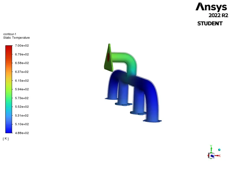
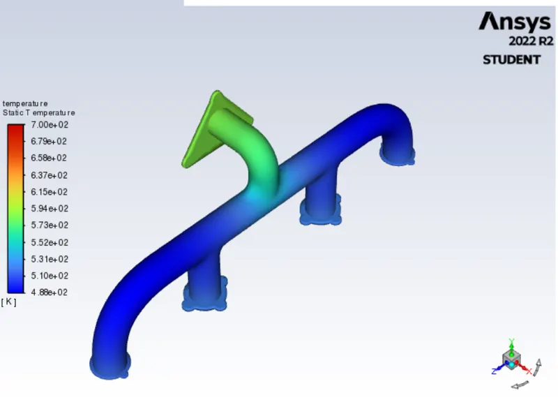
Temperature contour

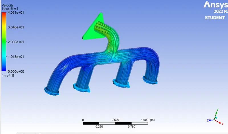
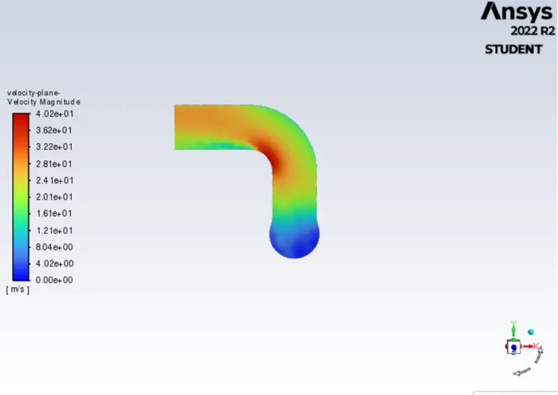
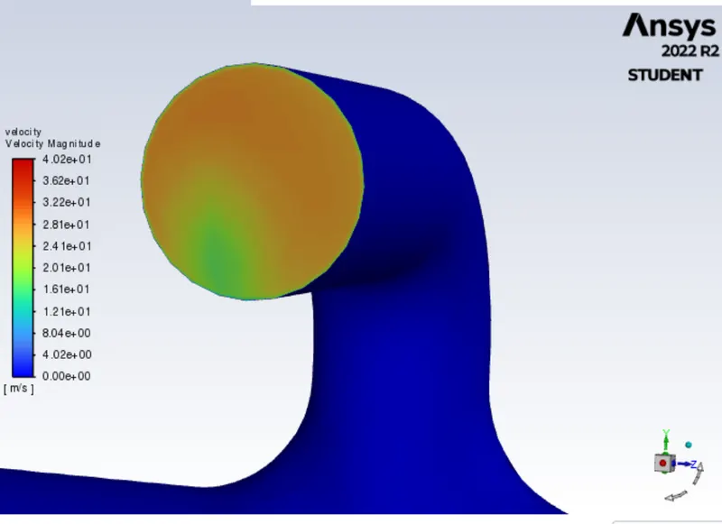
Velocity contour

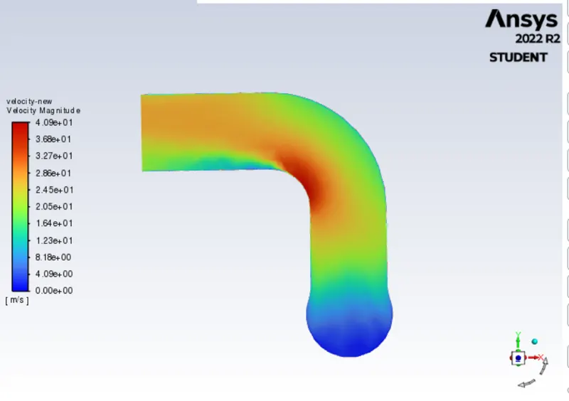
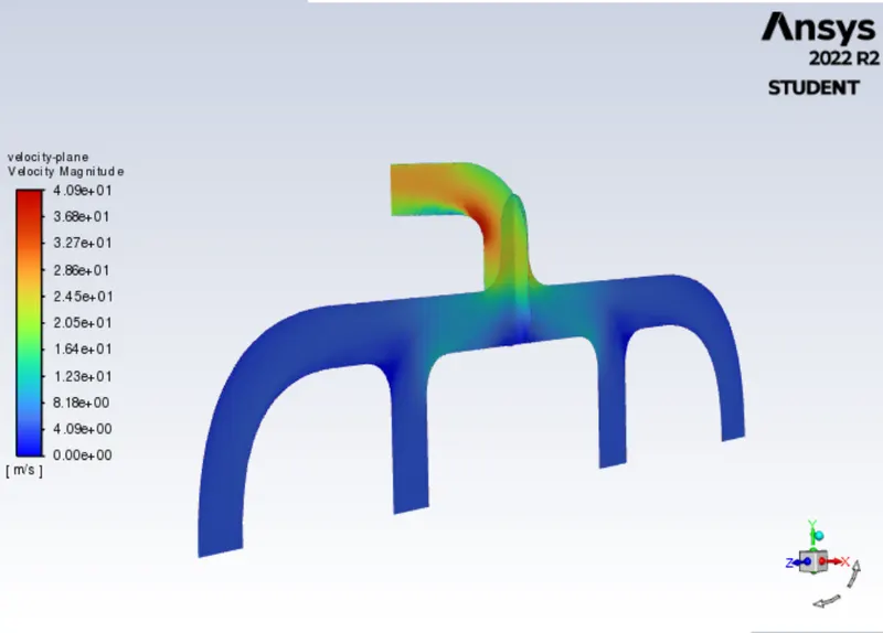
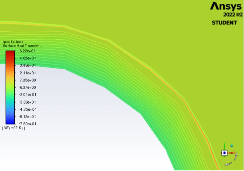
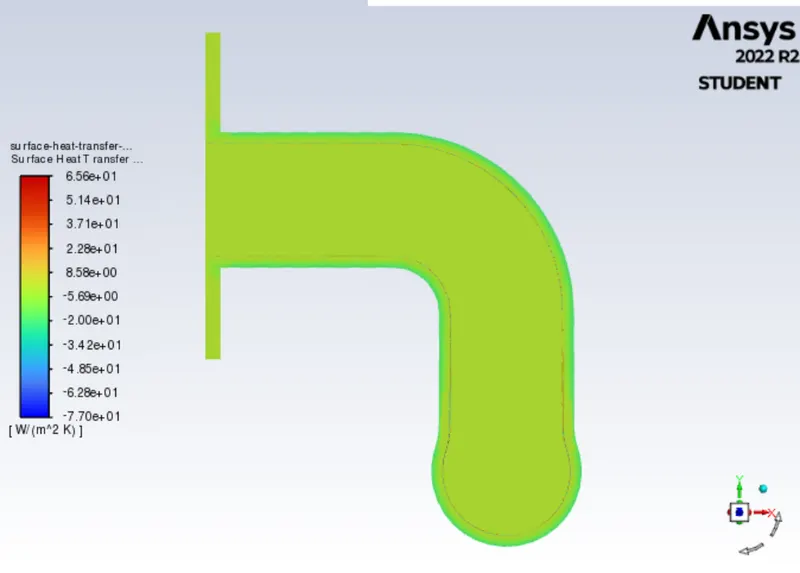
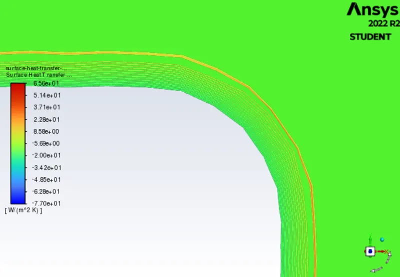
Surface heat transfer coefficient plot & contour

Case 2) 50mm

Here we are analyzing if any major changes appear if we give the finer mesh so we are giving the mesh element size smaller than the case 1. The geometry of the cases is similar so we are going to duplicate case 1.

Click the mesh option in the side window, select the sizing of mesh the element size as 50mm for outer surface and giving the inflation layer as 10mm. Here we have got the nodes (112358) and total elements (317167).

SETUP

In setup fluent check the given conditions are same as case 1. and click on initialize and click run iterations for 150 times after running create the planes for better analyzing the values.

Results

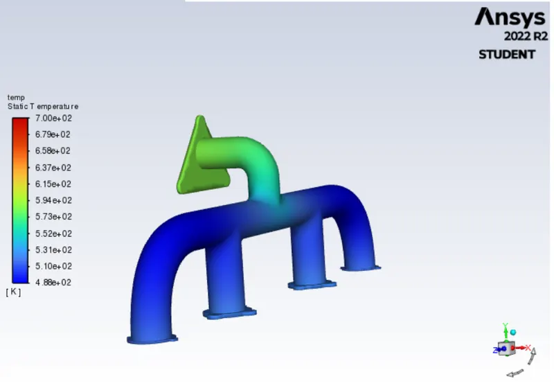
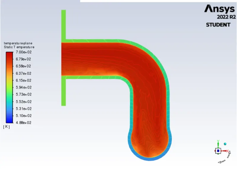
Temperature contour

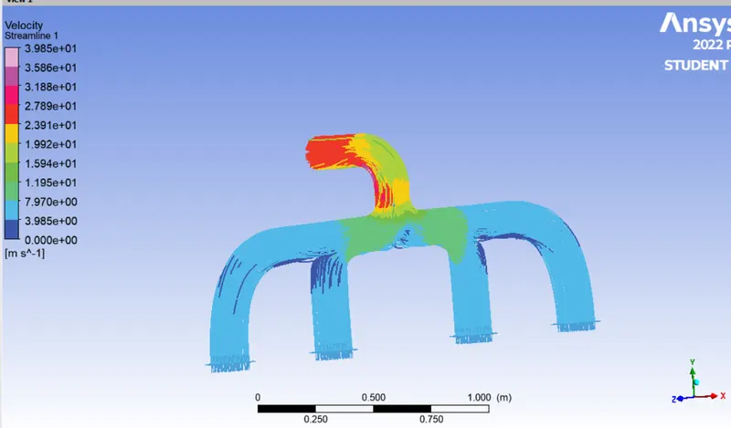
Velocity contour

Surface heat transfer coefficient plot

Case 3) 30mm

Here we are analyzing if any major changes appear if we give the finer mesh so we are giving the mesh element size smaller than the case 1 & 2. The geometry of the cases is similar so we are going to duplicate case 2.

Click the mesh option in the side window, select the sizing of mesh the element size as 30mm for outer surface and giving the inflation layer as 10mm. Here we have got the nodes (112464) and total elements (317411).

SETUP

In setup fluent check the given conditions are same as the case 1 and 2. and click on initialize and click run iterations for 150 times after running create the planes and contour plots for better analyzing the values.

Results

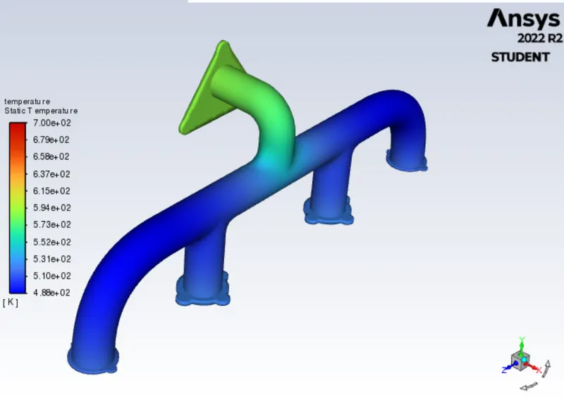
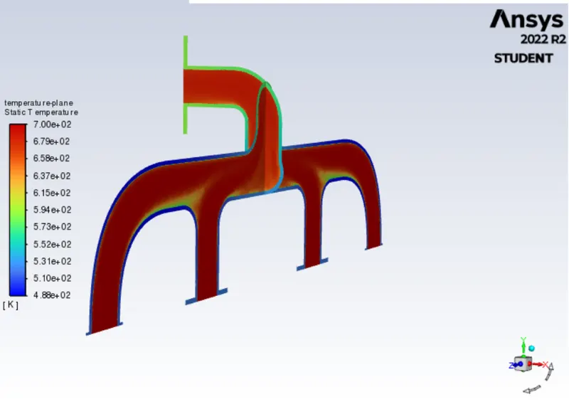
Temperature contour

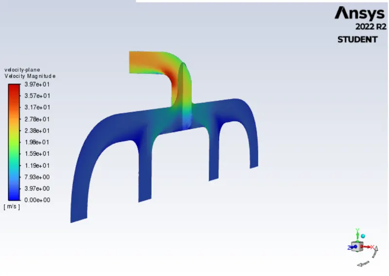
Velocity contour

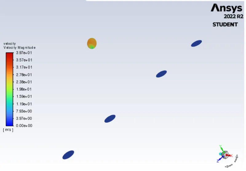
The below plot shows the velocity in inlet and outlet

Surface heat transfer coefficient plot

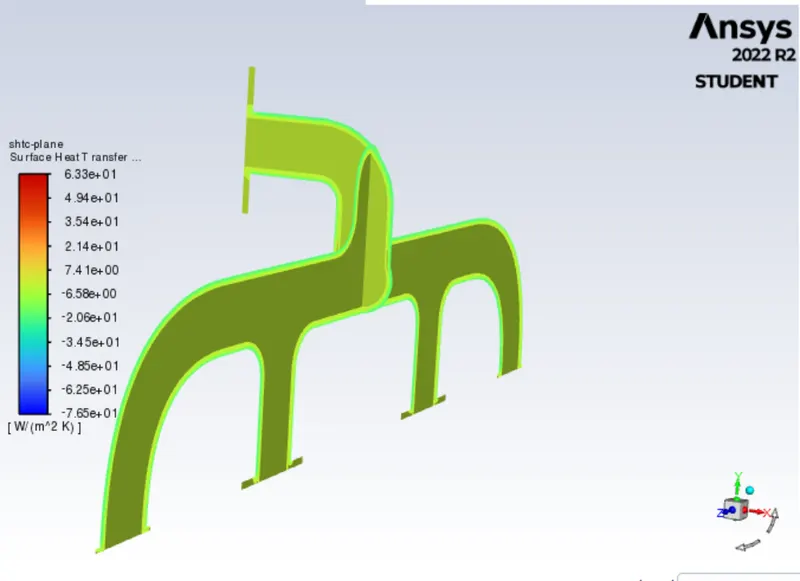
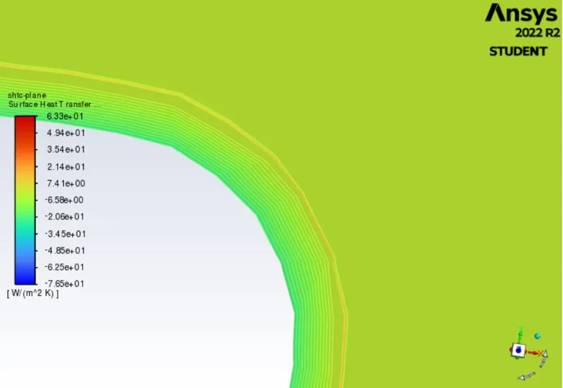
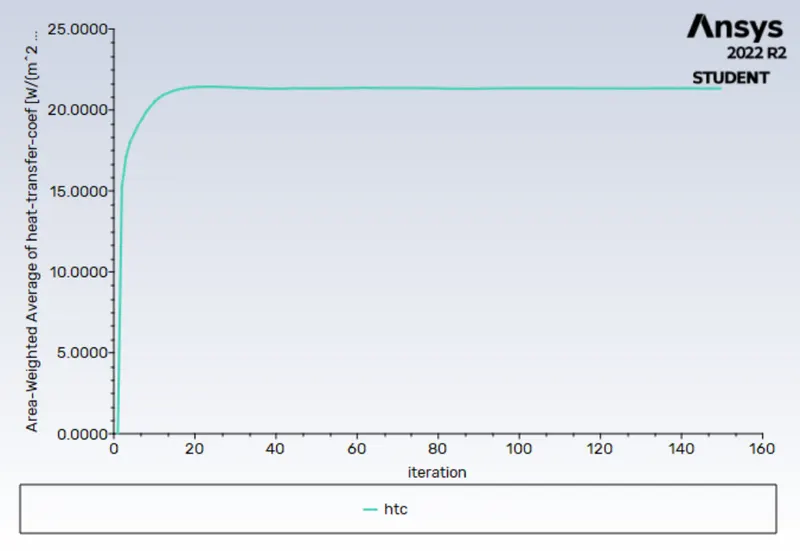
Refinement Mesh Nodes Element Heat Transfer Coefficient

1st refinement 150 86195 244906 21.347

2nd refinement 50 112358 317167 21.334

3rd refinement 30 112464 317411 21.327

VERIFYING HTC PREDICTIONS

The Nusselt number is the ratio of convective to conductive heat transfer across a boundary.

Nu_D = 0.023Re_D^4/5prⁿ

Were,

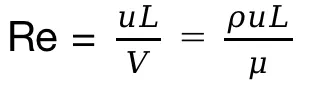
and u is the flow speed (m/s)

So, if you observe heat transfer coefficient is directly proportional to the Reynolds number (also to the velocity). So if you increase the velocity then there
will increase in the convective heat transfer coefficient. That's what we have proved above and if you want you can run another simulation by
increasing the Reynold's number of the flow then you will observe there will be increase in the overall convective heat transfer coefficient or at a particular
location than in the previous low Reynold's number simulation.

Factors that affect accuracy of the prediction:

• Accuracy of the geometric model – A precisely modeled geometry gives more accurate results.
• Wall thickness and other parameters like surface area of the geometry.
• Share topology – If this is not enabled, then the information between the solid and fluid surfaces are not shared properly.
• Mesh quality.
• Inflation layers.
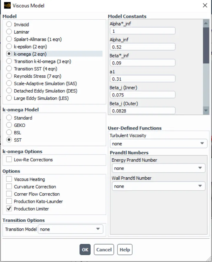
• Type of solver and turbulence model used.
• The type of fluid and solid materials used and its properties.
• Heat transfer co-efficient value.

CONCLUSION

The conjugate heat transfer analysis of the exhaust port has successfully been carried out and the respective temperature and velocity contour plots have been obtained from the simulation.

From the temperature contour plots, we can observe that the surface temperature of the exhaust port is higher near the outlet, as compared to the inlet, where the hot fluid enters through. We might assume that the surface is going to be the hottest at the inlet but it is infact the opposite. This is because of the phenomenon of convection.

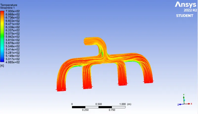
From the velocity contour graphs, we can observe that the fluid velocity is higher near the outlet, as compared to the provided velocity value at the inlet. This is due to the conservation of mass. The air from 4 inlets merge into a single inlet and therefore, the velocity is higher at the outlet. Finally, we can conclude that the flow velocity is directly proportional to the heat transfer co-efficient. Thereby, higher velocity leads to higher heat transfer co-efficient and hence leading to more heat transfer from fluid to the solid surface.