Week 4 - CHT Analysis on Exhaust port

Aim:

To run simulation to anlyse Conjugate Heat transfer in Exhaust port.

Abstract:

Conjugate heat transfer analysis plays an important role in predicting the thermal performances and effectively capture the boundary effect. In this case study an exhaust manifold is analyzed using CHT approach to predict the heat transfer coefficient value at the interface of the boundary wall of two different domain. Using k-omega turbulent model the capture of boundary effect is taken accurately and also the factors that account for better HTC prediction.

Objective:

1.To understand why and where a CHT analysis is used.

2.Run the CHT simulation using different turbulence model and justify results.

Introduction: Conjugate heat transfer analysis is based on a mathematically structured problem, which describes the heat transfer between a body and a fluid flowing over or inside it as a result of interaction between two objects. At the matching interface, the details are provided for temperature distribution and heat flux along the interface eliminating the need of calculating the heat transfer coefficient. Moreover, the heat transfer coefficient can be calculated later.

One of the simplest ways to realize conjugation is through numerical methods. The boundary condition for the fluid and solid interface is set and solved through iteration methods. There are no right guesses for the values of the initial boundary condition for the convergence except through the hit and trial method.

Application: The conjugate heat transfer methods have become a more powerful tool for modeling and investigating nature phenomena and engineering systems in different areas ranging from aerospace and nuclear reactors to thermal goods treatment and food processing from the complex procedures in medicines to ocean thermal interaction in metrology.

CHT in recent years has significantly improved the cooling performance of electronic equipment such as the design of heat sinks and the design of heat exchangers for the waste treatment plant. One such application of CHT is the exhaust port system.

Heat transfer coefficient (h):

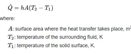
The heat transfer coefficient , in Thermodynamics is the proportionality constant between the heat flux and the thermodynamic driving force for the flow of heat

the heat transfer rate is:

Solving and modeling approach

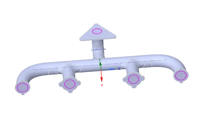
• The exhaust port was modeled into the Spaceclaim.
• The exhaust port is a three-dimensional model containing four inlets and one outlet. Despite having isothermal boundary conditions and a uniform flow rate at the four inlets, the model cannot be cut into two halves to save computational time because of its asymmetrical nature. Therefore the whole model is discretized and is considered for meshing.
• CHT analysis requires both the solid and the liquid volume under consideration, Spaceclaim gives an option of volume extract for selecting edges for fluid volume.
• Both the solid volume and liquid volume are copied into one component.
• Share topology is created.
• Spaceclaim gives an option for share coincident topology, when share coincident topology is selected and executed, the mesh from the fluid volume and the solid volume are said to be conformal with each other which is a requirement for CHT analysis.
• The exhaust port is loaded into the meshing window and then simulated for baseline mesh and the refined mesh.
• The named selections are created ( inlet, outlet, outer wall convection)
• The necessary contour images and graphs are studied to understand the behavior of temperature, velocity, and surface heat transfer coefficient at the interface.

Pre-processing and solver setting:

The geometry is loaded into Spaceclaim

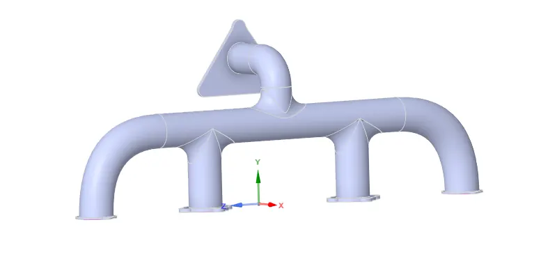
Fluid volume extraction:

It is the process of extracting the fluid volume from the solid volume.

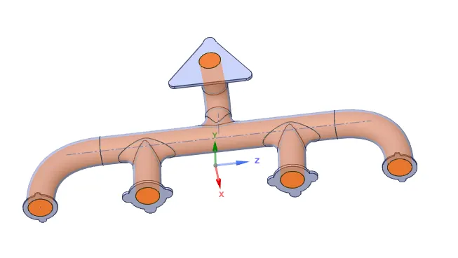
Share topology:

It is the process of sharing information from fluid volume to solid volume. It plays important criteria in CHT analysis.

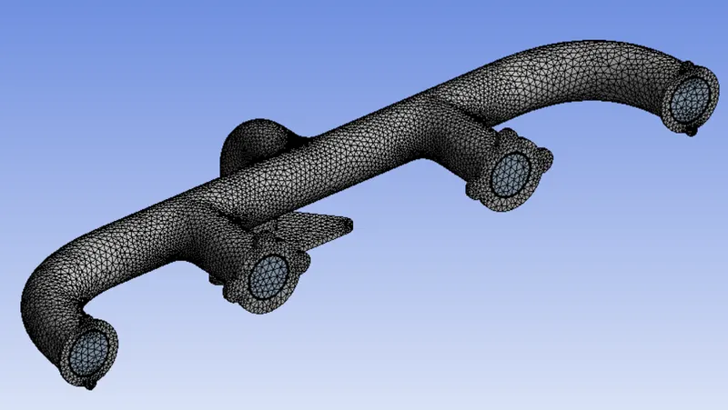
Meshing: It is the process of discretizing the geometry into a small number of volumes containing nodes. Since the geometry is complex and the mesh is unstructured therefore the finite volume scheme is used as a discretization scheme.

In this case, the default element size of ANSYS-FLUENT is used (0.15m).

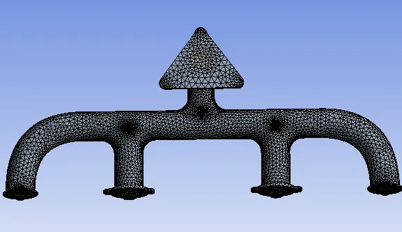
Mesh quality:

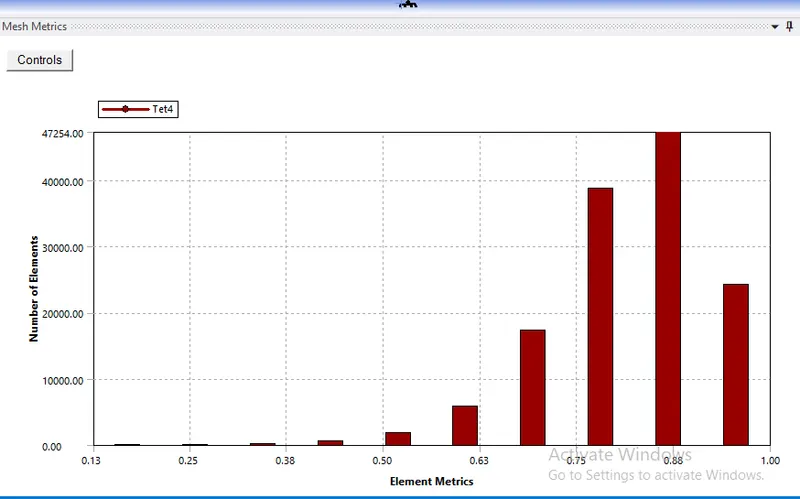
Mesh statistics:

Number of elements	135747
Number of nodes	27104

Named selection:

Inlet boundary condition (velocity inlet) @ 5msec

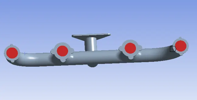
Outlet (Pressure outlet) Gauge pressure "0Pa"

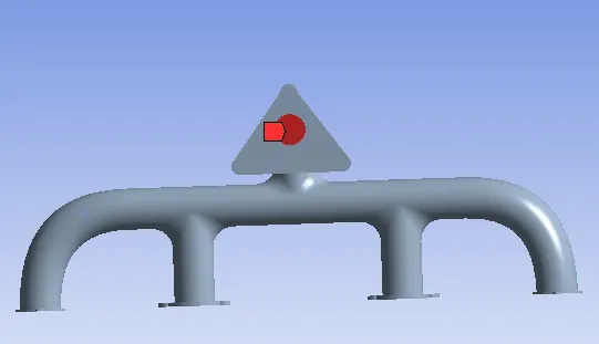
Outer wall convection (Heat transfer coefficient "20W/m2k"free stream temperature "300K")

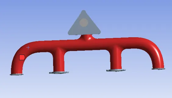
The flanges around the inlet and the component encompassing the outlet are adiabatic (no heat transfer takes place through these walls).

Solver:

Solver: Presure based steady state solver.

Refference Values:

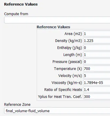
Boundary Conditions:

Inlet:

Velocity = 5 m/s

Temperature = 700 K.

Outlet: Pressure = 0 Pa (Gauge pressure)

Outlet wall convection:

Thermal condition: Convection

Heat transfer coefficient = 20 W/m2K.

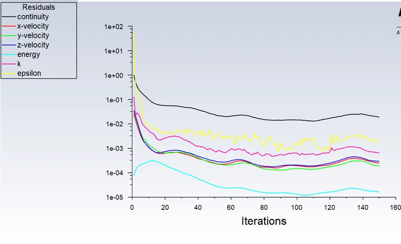
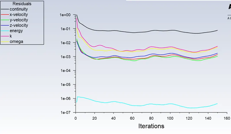
Simulation is ran for 150 iterations.

Results:

Case 1:

Mesh Size: 100 mm

Body sizing: 20 mm

Solver: K-epsilon standard

Mesh:

Residue Plot:

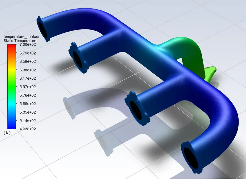
Temperature Contour:

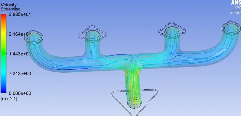
Velocity Steamlines:

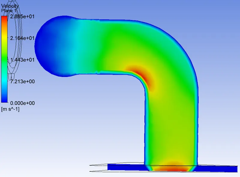
maximum velocity is 28.85 m/s and maximum velocity occured at outlet port.

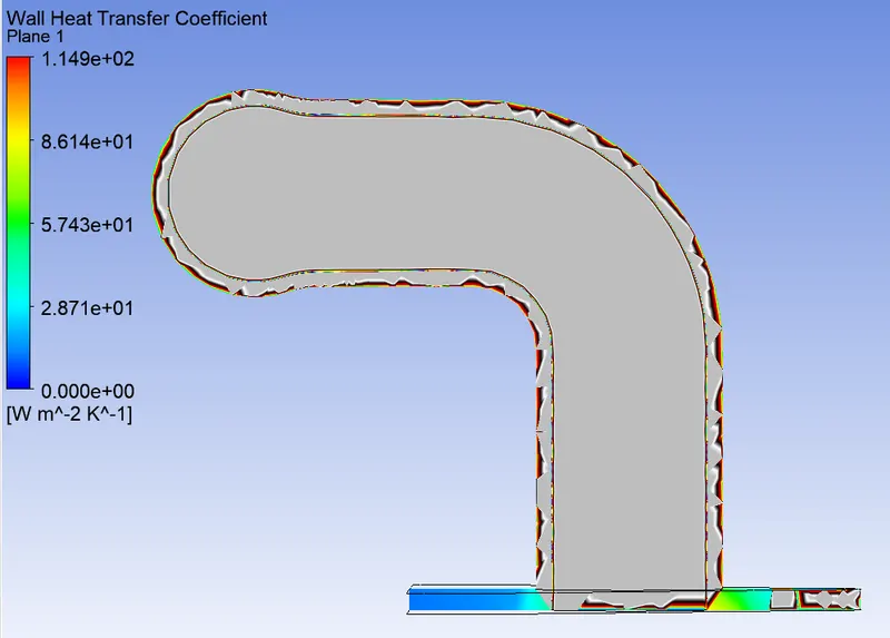
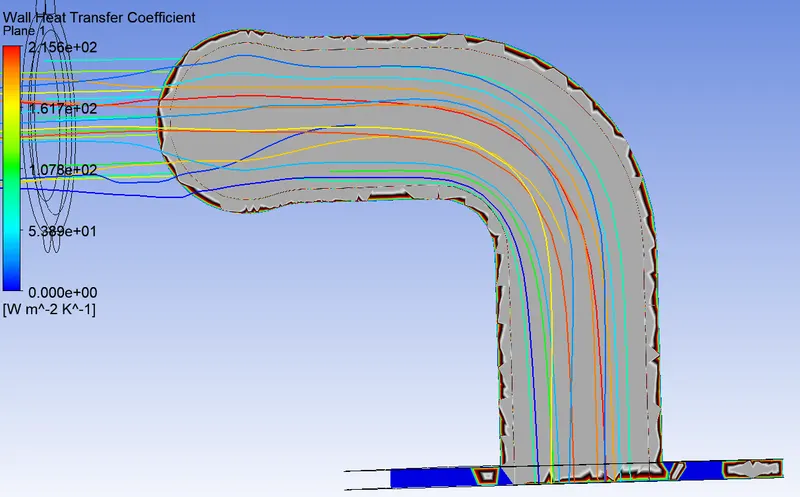
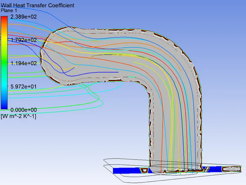
Wall Heat transfer coefficient:

Case 2:

Mesh Size: 100 mm

Body sizing: 20 mm

Solver: K-epsilon Reliazable

Mesh:

Residue Plot:

Temperature Contour:

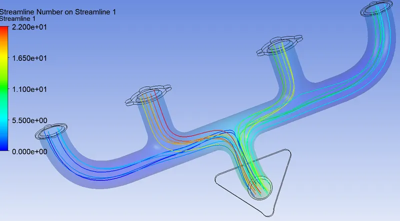
Velocity Steamlines:

maximum velocity is 22.00 m/s and maximum velocity occured at outlet port.

Wall Heat transfer coefficient:

Case 3:

Mesh Size: 100 mm

Body sizing: 20 mm

Solver: K-Omega

Mesh:

Residue Plot:

Temperature Contour:

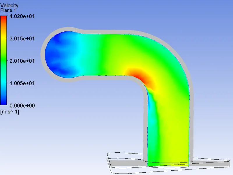
Velocity Steamlines:

maximum velocity is 40.20 m/s and maximum velocity occured at outlet port.

Wall Heat transfer coefficient:

Result Discussion:

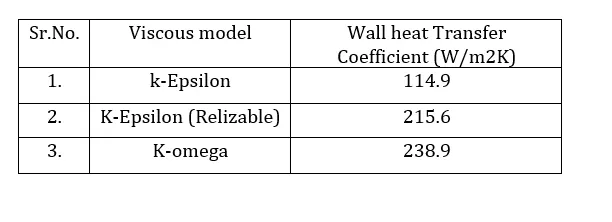
Wall heat transfer coefficient fro different viscous model is tabulated as follow:

• No difference in Temperature contours for all three viscous model is observed.
• Maximum heat transfer coefficient is found at layer adjacent to where maximum velocity is found.
• Maximum wall heat transfer is found using k-omega viscous model.

Conclusions:

1. The conjugate heat transfer analysis is successfully performed in two cases viz baseline and refine setup.
2. The maximum velocity for baseline case is found to be m/s and for refined case the maximum velocity is found to be m/s.
3. The wall y+ value as predicted from the k-omega model lies accurately within the range 0-5.
4. For the refined case setup, the heat transfer coefficient values is found to be 885 at the junction between the fluid and the solid boundary wall.