CHT Analysis on Exhaust port

Aim:-

• Brief Study on CHT analysis with why and where its uses.
• Calculate the Y+ value according to the turbulence model and simulate the final results.
• Calculate the wall/surface heat transfer coefficient on the internal solid surface.
• Also, plot velocity and Temperature contours on the required area.
• Confirm, if the HTC prediction from the simulation is correct. Furthermore, state, on what factors does the accuracy of the prediction depends.

Objectives:-

• Understand the concept of the Conjugated heat transfer along with its applications.
• Prepare the geometry by generating fluid volume. In this case, we will require both fluid and solid volume to calculate the heat transfer coefficient between fluid and solid.
• Simulate the baseline simulation to get an idea about simulation setup and results.
• For the final result execute a fine mesh with proper inflation layer considering proper Y+ value.
• Simulate with both k-epsilon and k-omega turbulent models to check suitable simulation types.
• Plot both wall and surface heat transfer coefficient on the internal solid surface.
• Plot velocity and pressure contour on the required area of the exhaust port.
• Validate the results with mesh independence and get confidence over results by conducting some exact calculation at the inlet and outlet port.
• State the factors of prediction that depend on the accuracy.
• Lastly, Write a brief report on the overall project.

CONJUGATE HEAT TRANSFER ANALYSIS

The Conjugate Heat Transfer (CHT) analysis type allows for the simulation of heat transfer between solid and fluid domain by exchanging thermal energy at the interface between them.

In solids, conduction often dominates whereas, in fluids, convection usually dominates.

Typical applications of this analysis type exist as, but are not limited to, the simulation of heat exchangers, cooling of electronic equipment, and general-purpose cooling and heating systems.

HEAT TRANSFER BY SOLID AND FLUIDS

Heat transfer in a Solid

In most cases, heat transfer in solids, if only due to conduction, is described by Fourier’s law defining the conductive heat flux, q, proportional to the temperature gradient:

`q=-k Delta T`

For time-dependent problem, the temperature field in an immobile solid verifies the following form of the heat equation:

`rho C_p (del T)/(delt) = Delta . (k.DeltaT)+Q`

Heat Transfer in a Fluid

Due to the fluid motion, three contributions to the heat equation are included:

• The transportation of fluid implies energy transport too, which appears in the heat equation as the convective contribution. Depending on the thermal properties of the fluid and on the flow regime, either the convective or the conductive heat transfer can dominate.
• The viscous effect of the fluid flow produces fluid heating. These terms in often neglected, nevertheless, their contribution is noticeable for fast flow in viscous fluids.
• As soon as a fluid density is temperature-dependent, a pressure work term contributes to the heat equation. This accounts for the well-known effect that, for example, compressing air produces heat.

According to these contributions, in addition to conduction, results in the following transient heat equation for the temperature field in a fluid:

`rhoC_p(del T)/(del t) + rho C_p u.del T = alpha_p T ((del p_A)/(del t) + tau . S + Delta . (k Delta T)+Q)`

After knowing what exactly Conjugated Heat Transfer (CHT) is, let us perform CHT analysis on the Exhaust port by using Ansys fluent

Fluent Analysis:-

Open Ansys workbench and drag and drop fluent setup cell in the Project schematics. Here we are going to perform three simulations. The first one, baseline simulation. In baseline simulation, we will get an idea about how the simulated results with coarse mesh will look like and where we will need fine mesh. It will also provide us parameters to calculate the y-plus value which is an important parameter to calculate the first inflation layer height and number of layers with total thickness.

For all the above results, we will refer to mesh for final simulations which are for K-epsilon and k-omega. And then, we will simulate our final results. And lastly, we will compare it to verify the dependency of the result.

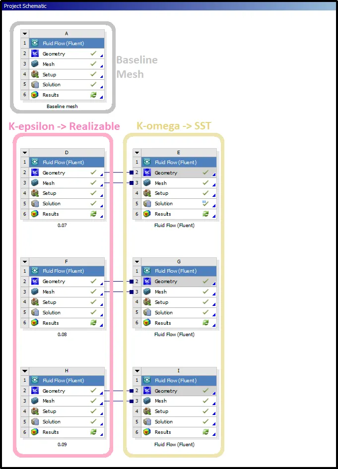
After creating the Fluent cell in the Project schematics, open design modeler to prepare geometry for fluent CFD simulation and import the geometry of the Exhaust Port.

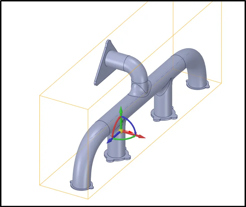
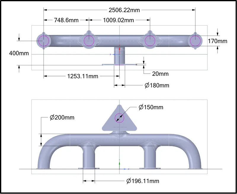
Geometry dimensions:-

Imported geometry is a solid CAD part, for fluent we need to create fluid volume to represent the fluid flow. To do that, go to Prepare --> click on Volume Extract --> Activate edge selector and select all the open edges --> click on the green checkmark.

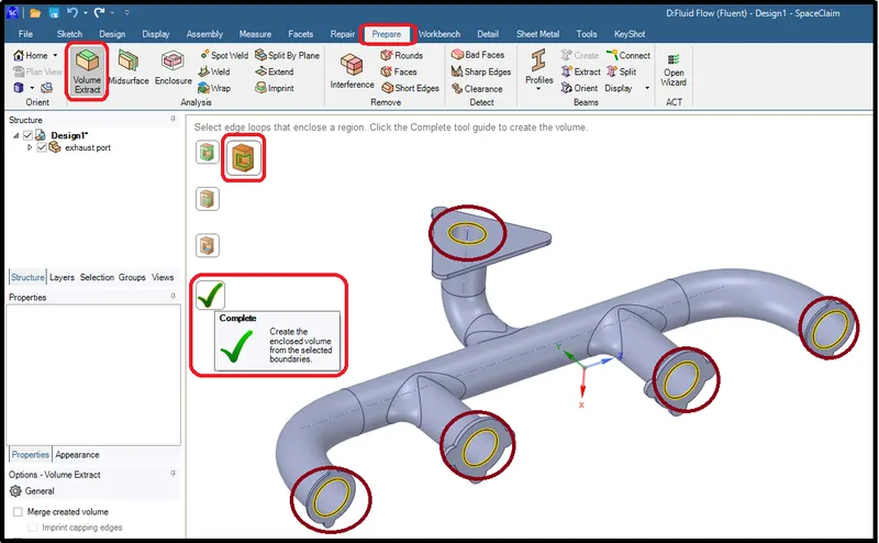
It will generate fluid volume inside the exhaust port as represented in the below figure

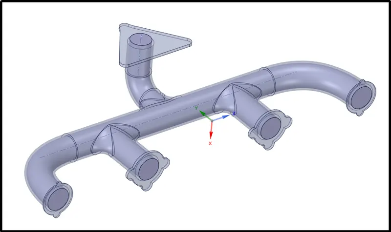
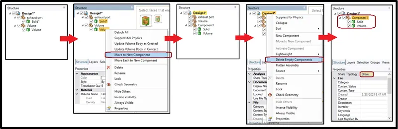
Here, we have two parts under the different components. To share geometry topology we required both parts in the same component. Simply select both parts and right-click. It will show ‘Move to the new component option’. select it and it will create a new component with the above-mentioned parts.

But now, we have two empty components. To delete it, Right-click on the main geometry name and select ‘Delete Empty components’.

Next, click on the new component, and in the topology option use share topology.

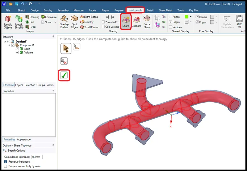
We also have to share geometry surfaces. Go to workbench --> select ‘Share’. it will show user-connected faces in red automatically. Simply click on the green checkmark to share faces.

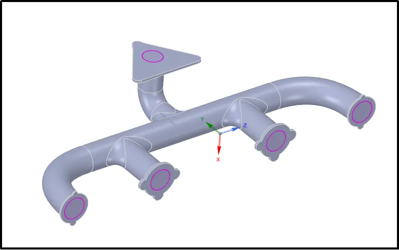
The final model prepared in space claim in space claim will look as depicted in the below figure.

Baseline Mesh:-

Before meshing first define the inlet, outlet, and other wall surfaces.

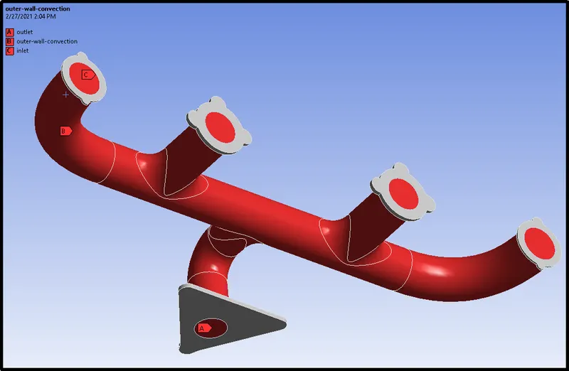
To generate baseline mesh, simply use the default mesh generated by a fluent meshing setup.

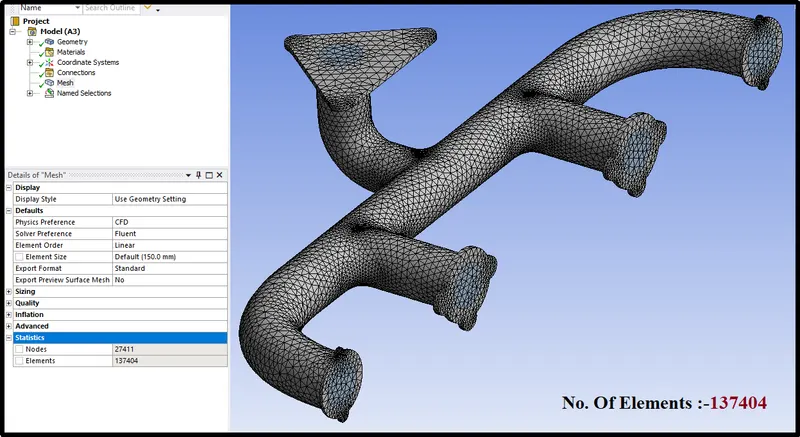
SIMULATION:-

For simulation, open the Fluent setup.

Simulation Setup:-

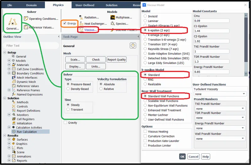
General Setting

Solver type --> Pressure based solver

Velocity formulation --> Absolute

Time --> Steady

Turn on the energy equation because we have to see temperature changes in CHT

Use k-epsilon turbulent Viscus model with standard wall function.

Material:-

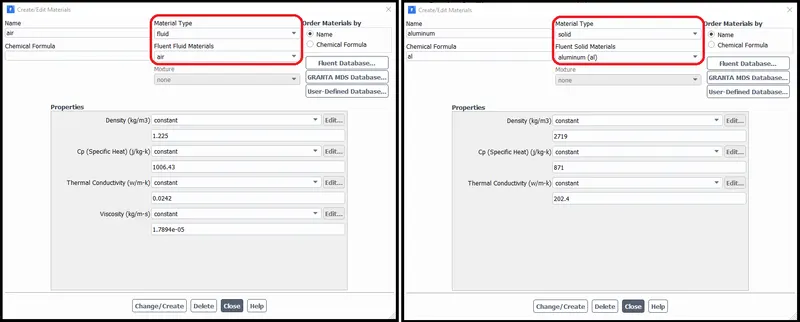
We are going to use fluent default material for fluid: air; for Solid: Aluminium

Boundary Condition:-

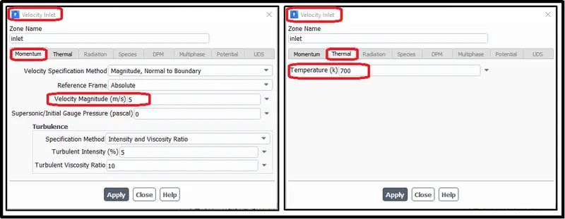
Define fluid velocity inlet as 5m/s with inlet temperature 700k.

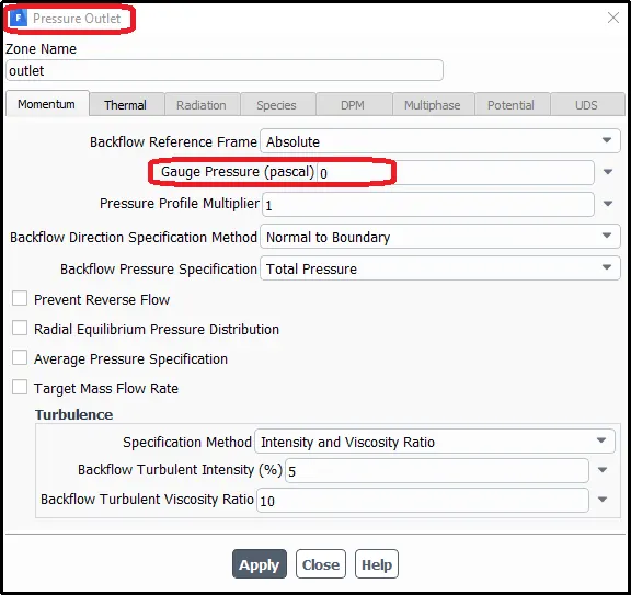
Outlet pressure will be the atmospheric pressure means zero gauge pressure.

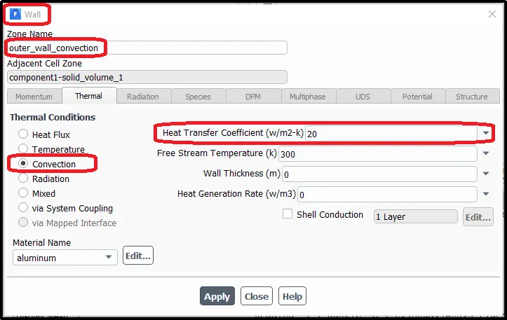
Outer wall surface

We are checking convection in this problem so select convection and provide the Heat transfer coefficient as 20w/m²-K. This value actually comes from the related reference data or by running a separate CFD simulation for it.

For this case lets just take this value from the skill Lync video tutorial of Exhaust port Simulation part1

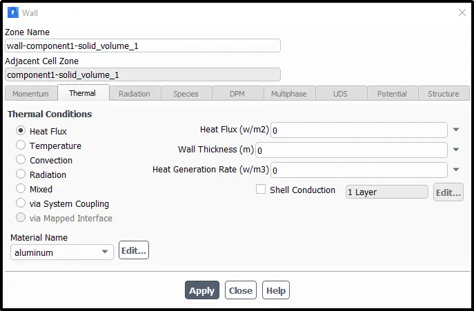
The remaining walls boundary condition

We are going to define adiabatic boundary conditions for other walls by setting the heat flux value as zero.

Initialize the setup - Hybrid initialization

The hybrid Initialization method is an efficient method of initializing the solution based purely on the setup of the simulation with no extra information required. These methods produce a velocity field that conforms to complex domain geometries and a pressure field that conforms to complex domain geometries and a pressure field that smoothly connects high and low-pressure values.

Finally, run the setup for 400 iterations.

Residual plot:-

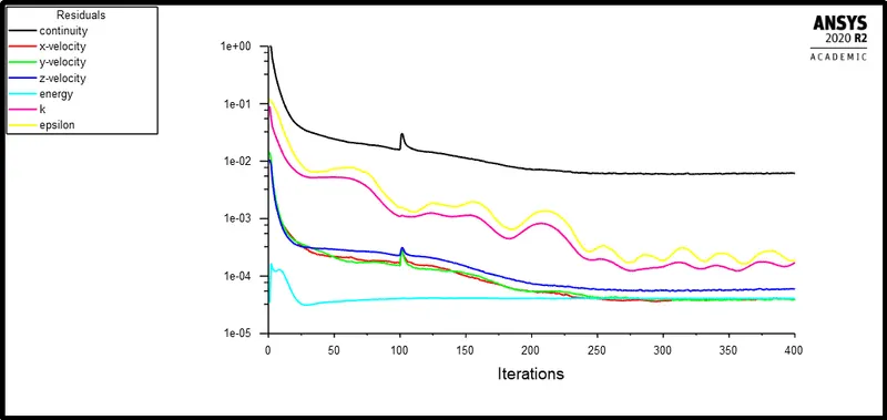
From the residual plot, for baseline mesh, we can assume our solution converged as the residuals are not showing any major changes with each iteration.

Results From Baseline mesh:-

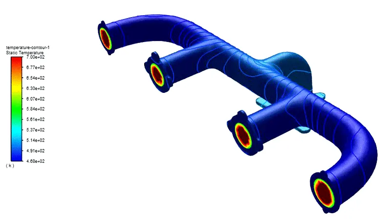
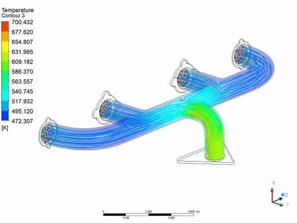
As above .gif image, we can see when all the stream merging at the outlet port the temperature is raising

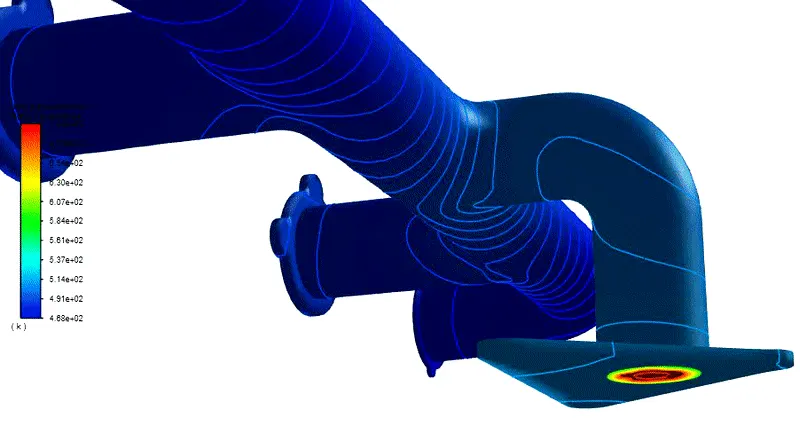
To see changes more clearly watch the above .gif file which showing the temperature changes near the outlet exhaust pipe. To see what exactly happening inside, we will create a cut plane at the center of the outlet exhaust port.

Wall heat transfer coefficient:-

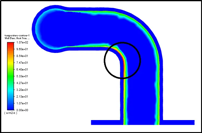
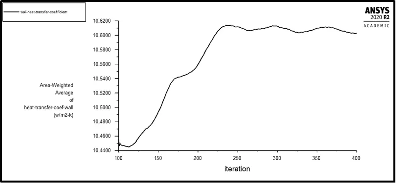
The wall heat transfer coefficient is the quantity calculated only near the walls which are adjacent to the fluid. And it is highest near the inner bent area as shown in the figure within a black circle. The reason for this phenomenon is because the velocity at this area is high.

We can observe the wall heat transfer in a nice magnified way when the wall adjacent mesh is coarse since it is calculated only on the mesh which is adjacent to the wall.

Velocity contour at outlet port:-

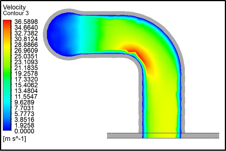
As above velocity contour plot demonstrates the velocity is maximum at the bent area to prove our above statement.

Velocity Streamline at outlet port:-

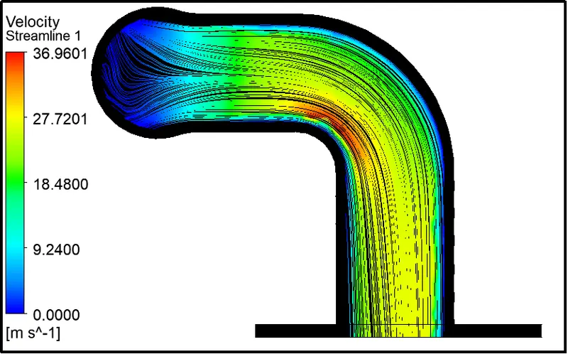
The maximum velocity in this simulation we are getting is 36.9601 m/s.

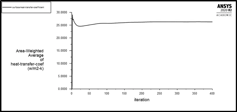
Surface heat transfer coefficient

Wall heat transfer coefficient

Wall Y+ Plot

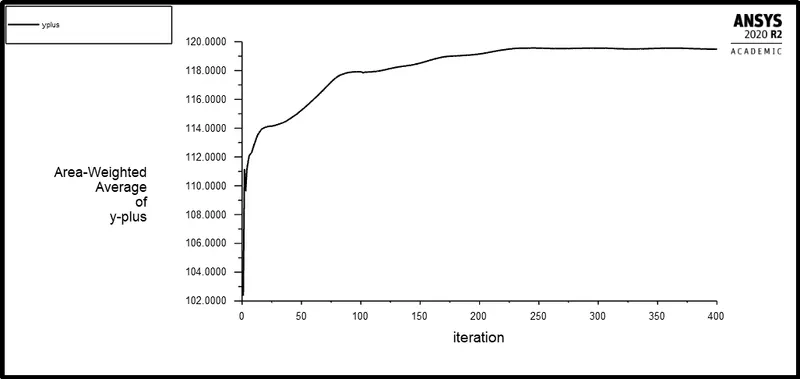
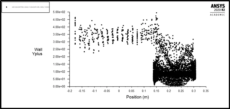
In the Y+ plot, we can notice the average Y+ value is 119 and the maximum y plus is near 500. This value that we got from the baseline simulation is very high. This means it is not capturing the flow near-wall surface with proper effectiveness. Therefore, we need refined mesh with proper y+ plus value for our final mesh.

Final Setup (k-epsilon):-

Geometry Setup:-

We are going to use the same geometry setup for the final simulation

Meshing:-

Y+ Boundary layer

The behavior of the flow near the wall is a complicated phenomenon and to distinguish the different regions near the wall the concept of wall Y+ has been formulated. Thus Y+ is a dimensionless quantity and is the distance from the wall measure in terms of viscous length.

In the turbulent boundary layer region flow near the wall has been analyzed in terms of three layers.

• The inner layer, or sublayer, where viscous shear dominates.
• The outer layer, or defect layer, where large-scale turbulence eddy shear dominates.
• The overlapping layer, or log layer where velocity profiles exhibit a logarithmic variation

One of the reasons for the need for Y+ is to distinguish different regions near the wall or in the viscous region, however, how exactly it helps in turbulence modeling or general CFD modeling needs to be well understood. If we intend to resolve the effects near the wall i.e., in the viscous sublayer then the size of the mesh size should be small and dense enough near the wall so that almost all the effects are captured. But in some cases, if the wall effects are negligible then there is the option of including semi-empirical formulae to bridge between the viscosity-affected region and fully turbulent region, and in this case, the mesh need not be dense or small near the wall i.e, the coarse mesh would work.

Considering the first case, i.e., near-wall modeling it is well-known that the mesh size should be small enough, however then the question following is how small? Thus, here comes the concept of Y+, and based on the Y+ value the first cell height can be calculated. The near-wall region is meshed using the calculated First Cell height value with gradual growth in the mesh so that the effects are captured and avoiding overall heavy mesh count.

Calculating the first Cell Height for a desired Y+ value

Firstly, we should calculate the Reynolds number for our model based on the characteristic scale of our geometry such that:

`Re = (rho.U.L)/mu`

Where,

`rho` is the fluid density

`mu` is the viscosity

U is the free-stream velocity,

L is the characteristic length

So, we are going to take max velocity near the outlet for consideration of free stream velocity in the calculation.

maximum free stream velocity = 5 m/s,

Density = 1.225kg/m^3,

Dynamic Viscosity = 1.7894e-05kg/ms,

For length consideration, we are going to consider length along x-Axis as shown in the below figure, which will give approx length value towards an outlet for Reynolds number calculation.

Length = 170mm = 0.170m (Inlet inner Diameter)

`Re = (1.225xx5xx0.170)/(1.7894e-5)`

`Re = 5.8190e+04`

The definition of the Y+ value is such that:

`Y+ = (rho.U_tau.Deltay_1)/mu --> Delta y = (Y+.mu)/(rho.U_tau)`

The wall shear stress, `tau_w` can be calculated from the skin friction coefficient, `C_f`, such that:

`tau_w = 1/2. C_f.rho.U^2`

The ambiguity in calculating `DeltaY1` surrounds the value for `C_f`. Empirical results have been used to provide an estimate to this value:

For internal Flow type --> Empirical Estimate (`C_f = 0.079. Re^-0.25`)

For External Flow type --> Empirical Estimate (`C_f = 0.058. Re^-0.2`)

Use `C_f` for internal flow,

`C_f = 0.079 xx (9.8667e+05)^-0.25 = 0.0051`

`tau_w = 1/2(C_f.rho.u^2)`

`tau_w = 1/2(0.0051)(1.225)(5^2)`

`tau_w = 0.0779`

Friction velocity

`U_f = (tau_w/rho)^0.5`

`U_f = (0.0779/1.225)^0.5`

`U_f = 0.2522`

Depending upon the turbulence model and the wall treatment, you can get different values from the computation for Y+ and friction, not always coherent with other theories or measurements.

To integrate the equations through the viscous/laminar Sublayer, a “Low Reynolds” approach must be employed. This is achieved as additional highly non-linear damping functions are needed to be added to low Reynolds formulations (Low as in entering the viscous/laminar sub-layer) to be able to integrate through the laminar sub-layer (Y+<5). This again produces numerical stiffness and in this case, is problematic to handle given linear numerical algorithms.

Now to get desired results we will consider the Y+ value as 1.5

Therefore, for Y+ = 1.5 first layer thickness

`Delta y = (1.5xx1.7894e-05)/(1.225xx0.2522) = 0.0000855m ~ 0.08mm or 0.09mm`

now, in this case, we are taking Y+ =0.08mm into consideration. If we do not obtain the desired thickness, then we do it by hit and trial way.

For the first layer thickness 0.08mm

Number of layers

n = 12

Growth rate

`Gr = 1.5;`

Total thickness

`T_t = Delta y *Gr^(n-1)`

`T_t = 6.9198mm`

For fluid boundary:- we use the total thickness of 6.9198mm with 12 inflation layers considering the growth factor as 1.5.

For solid boundaries:- we assume 6 boundary layers with 5mm total thickness considering 1.2 growth rate factor.

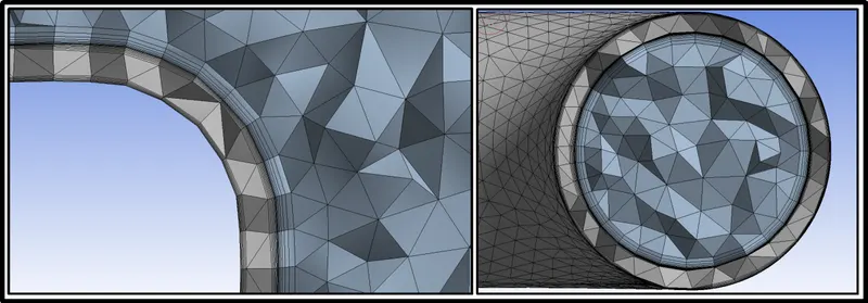
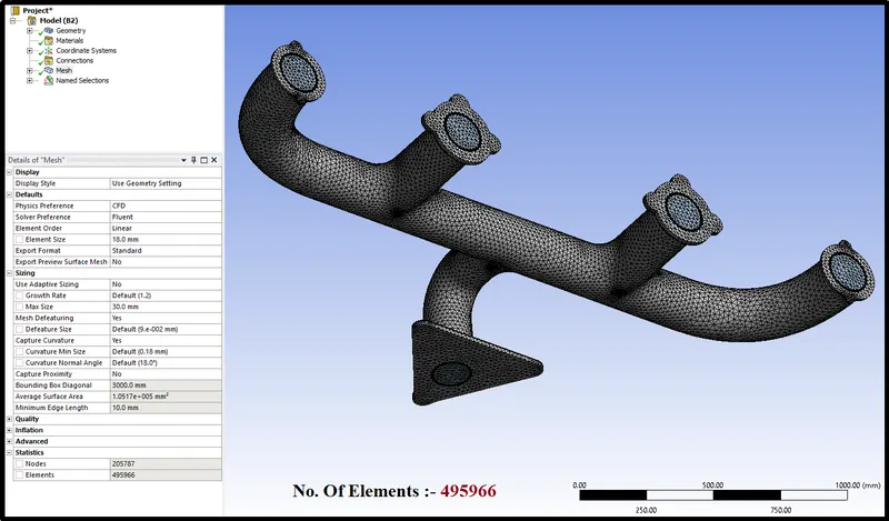
By defining the above mesh condition we will generate the mesh for the final simulation as shown in the below figure.

Fluent Setup:-

For very fine mesh, to calculate very fine mesh near-wall K-epsilon model with realizable is preferable. Because it calculates the results with the fine mesh neat wall without giving large fluctuations in values.

In the viscus model, select ‘k-epsilon’,’ Realizable’ for our first type of simulation. Turbulence modeling is a complex area. The choice of model depends on the application. Here, the Realizable k-epsilon model is used which is an improvement on the well-established standard k-epsilon model. Accept the remaining default settings.

We are choosing enhanced wall treatment as heat transfer coefficient results highly dependable on calculation near-wall surface. Additionally, we will also consider the pressure gradient effect, Thermal effect, and viscus heating in simulation.

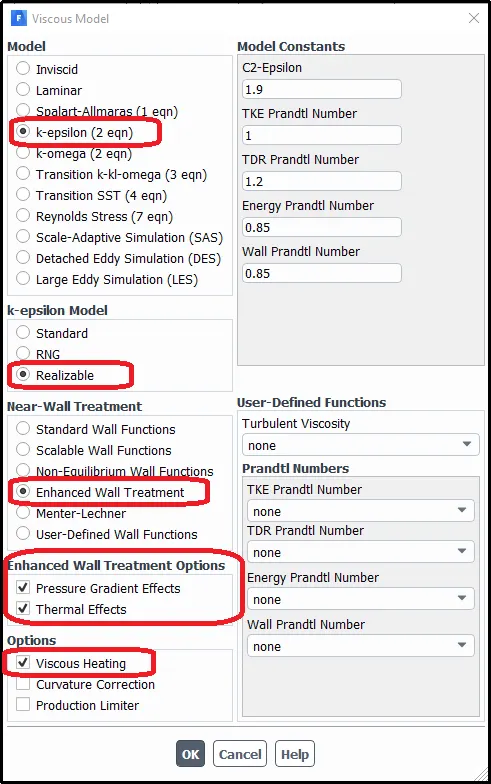
Remaining all the setup will be the same as the baseline simulation setup except for reference values.

In the fluent software, the value of the convective heat transfer coefficient extremely depends on the reference temperature. we should use the proper bulk temperature as the reference temperature. Therefore, we will provide an inlet reference temperature of 700k.

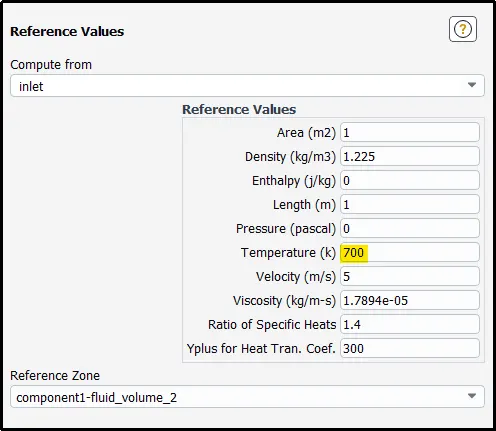
Finally, run the setup file for 500 iterations.

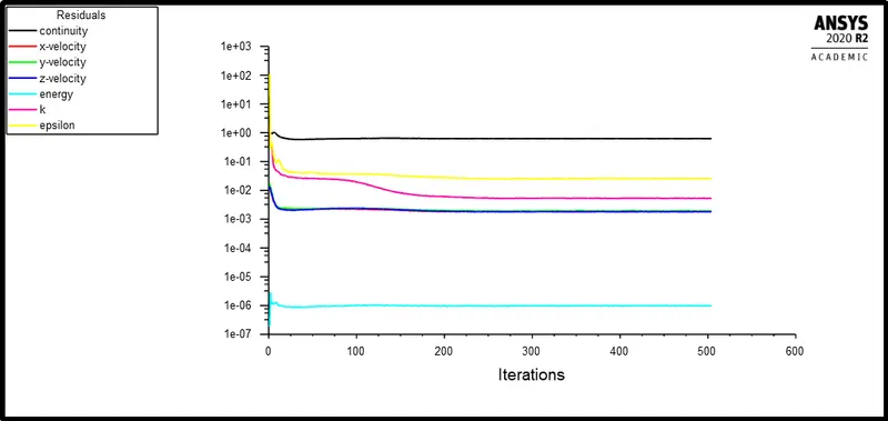
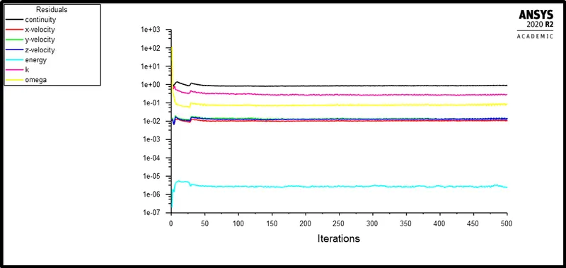
From the residual plot, for the final mesh, we can assume our solution is converged as the residuals are not showing any major changes with each iteration.

Results:-

Heat transfer coefficient:-

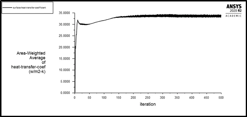
Average Heat Transfer Coefficient(W/m²-K) = 32.929 W/m²-K - 34.267W/m²-K

Y+ value

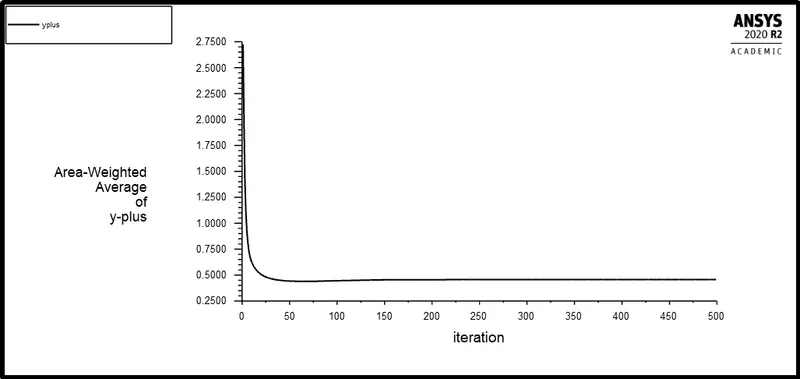
The average Y+ value is 0.28645772

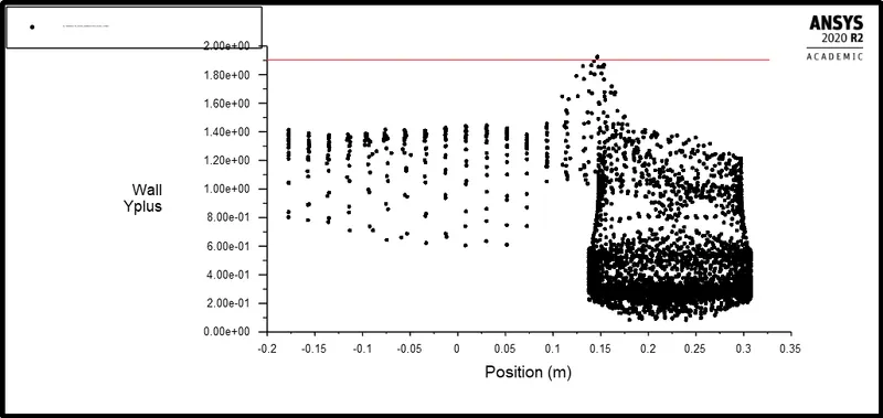
Bu the maximum Y+ value is showing neat 1.2 which is very close to 1 so we are going to accept this value.

Wall Heat transfer coefficient:-

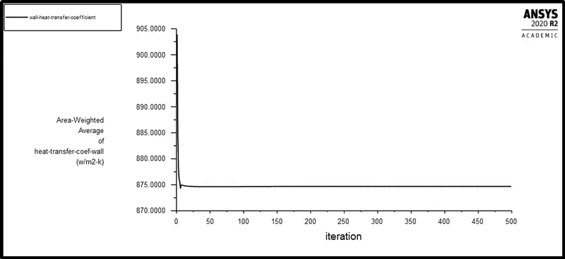
The average wall heat transfer coefficient for 0.08 first layer thickness is 874.93697W/m²-K.

The difference in-wall and surface heat transfer

Assume that there is a layer that is very close to the wall in either case of turbulent or laminar and that h (wall heat transfer coefficient) is very high compare to upper layer h which surface heat transfer coefficient.

Wall Heat Flux(q)W/m^2 = `hxx(T_(fluid) - T_(wall))`

So, that layer temperature is high and thus the difference is less which automatically make our h big at the wall and q is also big. The h calculate from formulas give us the surface heat transfer coefficient which is away from the wall.

Final Setup (k-omega - SST):-

For the K-omega setup, we are just going to make the following changes in our fluent setup rather than that geometry, mesh and everything else will be the same.

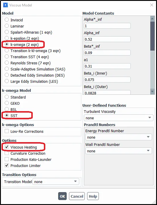
The k-omega (k−ω) turbulence model is one of the most commonly used models to capture the effect of turbulent flow conditions. It belongs to the Reynolds-averaged Navier-Stokes (RANS) family of turbulence models where all the effects of turbulence are modeled.

SST stands for shear stress transport. The SST formulation switches to a k-e behavior in the free-stream, which avoids the k−ω problem of being sensitive to the inlet free-stream turbulence properties.

The k−ω SST model provides a better prediction of flow separation than most RANS models and also accounts for its good behavior in adverse pressure gradients. It has the ability to account for the transport of the principal shear stress in adverse pressure gradient boundary layers. It is the most commonly used model in the industry given its high accuracy to expense ratio.

On the negative side, the SST model produces some large turbulence levels in regions with large normal strain, like stagnation regions and regions with strong acceleration. This effect is much less pronounced than with a normal k-epsilon model though.

We are going to run this setup for 500 iterations

Residuals plot:-

Results:-

Heat transfer coefficient:-

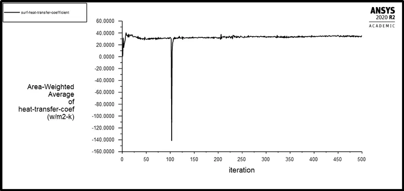
Average Heat Transfer Coefficient(W/m²-K) = 2.8786W/m²-K - 3.4035W/m²-K

Y+ value:-

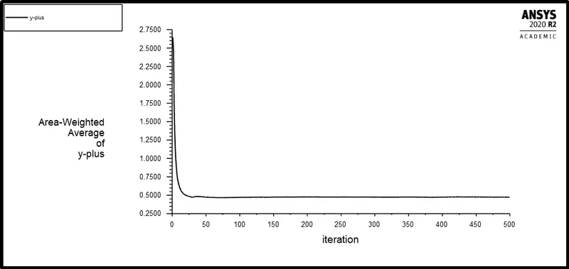
the average Y+ value is 0.28645772

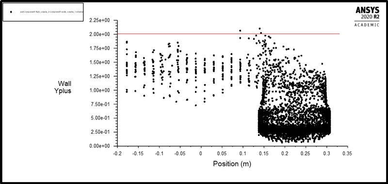
the maximum Y+ value is showing near 2. so, we are going to accept this value.

Wall Heat transfer coefficient:-

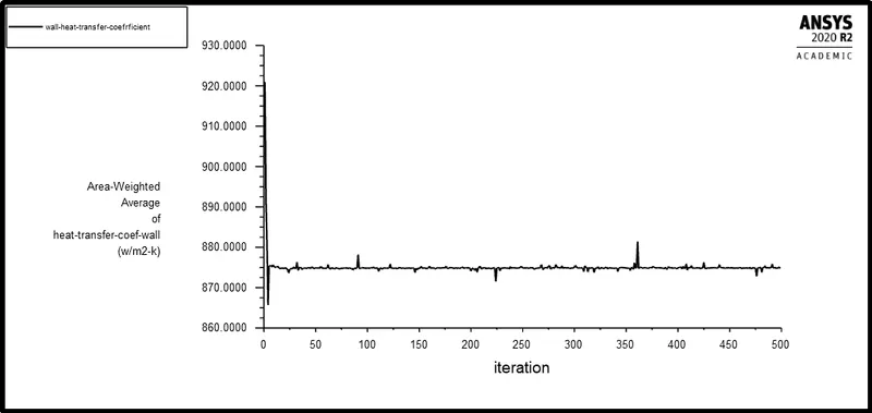
The average wall heat transfer coefficient for 0.08 first layer thickness is 874.93697W/m²-K.

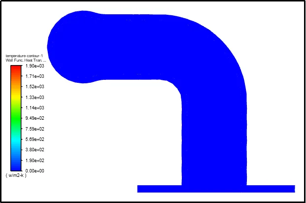
Because of the very small thickness of the inflation layer, it is very hard to notice the Wall thickness coefficient in the final simulation as the wall heat transfer coefficient is the quantity that can only be calculated near the wall that is adjacent to the fluid. To observe it properly different simulations had run with a 5mm thickness of a single inflation layer. And the following picture has been taken from that simulation result.

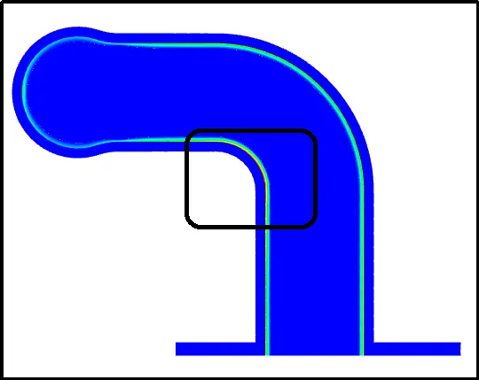
We can now observe the maximum wall heat transfer is located near the inner bent area. The following picture shows the magnified view of that area.

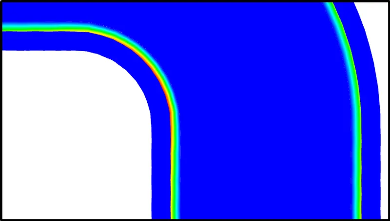
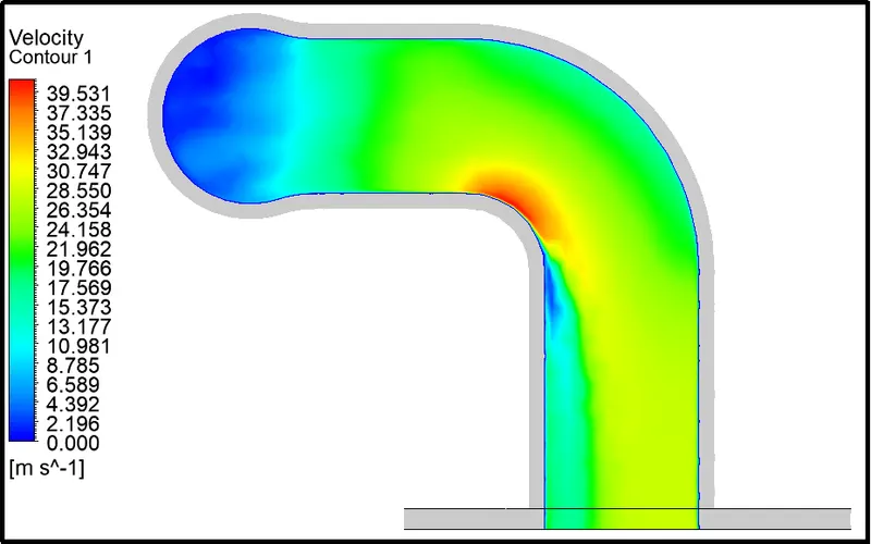
wall heat transfer coefficient is higher in the above-mentioned area because that is where the velocity also is highest. If on the same cut plane if we plot the velocity plot we can see that that's the region with the highest velocity. We can observe this in the below velocity contour plot.

Velocity Streamlines:-

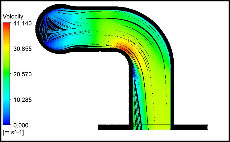
the highest velocity is 41.140m/s which is flowing through that particular region means a higher Reynolds number. That’s why the heat transfer coefficient in that area is highest, which means the maximum amount of heat transfer is taking place from fluid to the solid in that region. This also results in a higher temperature of solid in that location.

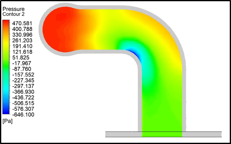
The reason for higher velocity is the pressure which reducing drastically near the outlet of the exhaust port. And because of sharp turn pressure is again reduce at the inner bent section of that pipe.

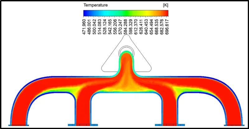
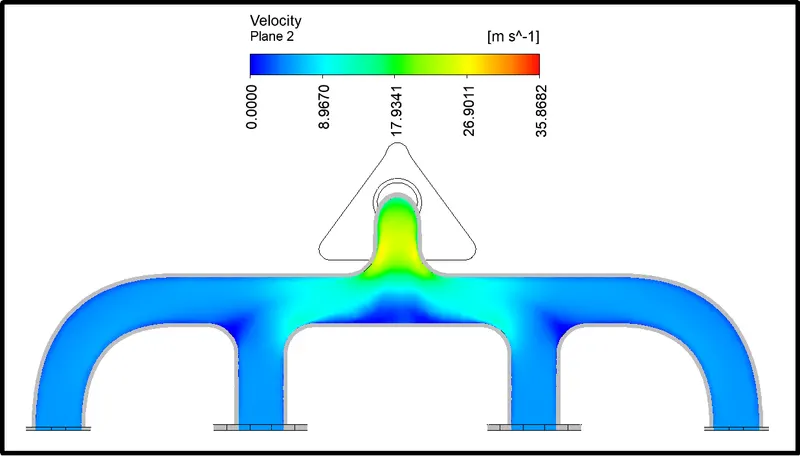
Additionally, we can see the region of high velocity in that region is all the velocity from different inlet ports are mixing there and coming out from the one single outlet. Hence the heat transfer coefficient is high from the merging region to the outlet.

Velocity Flow animation

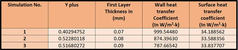
Wall and surface heat transfer on an internal solid surface:

K-epsilon -> Realizable

K-omega -> SST

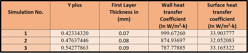
Validation of HTC value

In the above tables, the heat transfer coefficient is calculated for different mesh and different Y+ values to perform the mesh independency test. In each simulation, it is giving almost the same surface heat transfer value which is the actual (h) heat transfer coefficient.

We can also compare our results with analytical results

Heat transfer coefficient at the inlet

The heat transfer coefficient can be calculated as

`h = (k/D_H)xxN_u`

Where,

k is the thermal conductivity of the liquid = 0.0242,

`D_H` is the Hydraulic diameter

`N_u` is the Nusselt number

`N_u = 0.023Re^0.8P_r^n`

n = 0.3

where,

`Re` is the Reynolds number

`P_r` is the Prandtl number

`Re = 5.8190e+04` ( as we calculated earlier)

`P_r = (C_p*mu)/k`

`P_r = (1075xx1.7894e-05)`

`P_r = 0.7949`

`N_u = 0.023xx(5.8190e+04)^0.8xx(0.7949)^0.3`

`N_u = 139.2182`

`h = (0.0242/0.170)xx139.2182`

`h = 19.8181`W/m²-k

At the inlet, the velocity is very less which causes less heat transfer rate.

Heat transfer coefficient at the outlet

The average outlet velocity from the simulation is 25.278964m/s

Therefore, Reynolds's number will be...

`Re = (rho.U.L)/mu`

`Re = (1.225xx25.278964xx0.150)/(1.7894e-05)`

`Re = 2.5958e+05`

`P_r = (1075xx1.7894e-05)`

`P_r = 0.7949`

`N_u = 0.023xx(2.5958e+05)^0.8xx(0.7949)^0.3`

`N_u = 460.5124`

`h = (0.0242/0.170)xx139.2182`

`h = 74.2960`W/m²-k

At the outlet, the velocity is high which means a high Reynolds number which leads to a high heat transfer rate, therefore, higher heat transfer coefficients.

The above analytical problem refers to the heat transfer coefficient of simple pipe problems which never gives exact results for complicated geometry like exhaust port. But it gives the right intuition about the range of our results we are getting from the fluent simulation. So one can know their results are within the criteria.

Factor to get the best heat transfer coefficient value.

• Heat transfer coefficient is the function of properties of the fluid at film temperature, temperature difference, temperature coefficient, buoyance force, etc., hence, mesh resolution near the walls usually has the biggest impact on numerical results.
• Creating an inflation layer with a proper Y+ value near the fluid wall face is vital. For turbulent model, where capturing near-wall surface movement is important Y+ plus value should be less than 5 (Y+<5). for the most time, it should be near 1and 2.
• It is also greatly affected by the selection of the turbulent model. In such a case, the SST k omega model is preferable which resolves the flow near the wall.( For this the y+ =1). K-epsilon with some near-wall treatment (eg. enhanced wall treatment) options available in fluent, also works with refined meshes (Y+ ~1).
• Next, boundary conditions and material assigned in simulation should be correct. In the short simulation, the setup should be correct.
• Results should be validated by mesh independence to get a confirmation that results are not changing with different meshing.
• Finally, if possible it can be validated by analytical/ exact and experimental methods. But results got from all three methods may vary sometimes because of complicated shapes, some real-life factors which fluent did not take into consideration while simulating the problem, the accuracy of the measuring instruments used, the flow pattern, the equations used in the theoretical side, etc. Even though these results gave us the rough range that we can consider for verification.

Conclusion:-

• For the turbulent models, we have to take care of the assumptions and the boundary conditions we put in the program. The mesh is a very important parameter to get good results, that's why we have to refine it in the important place of our geometry.
• Some factors should be considered which the most significant is the turbulent boundary layer. If we are using any kind of low Reynolds turbulence model considering enhanced wall treatment (as our K-w SST model), so we need to make sure that we stay in the laminar sub-layer region where velocity profiles are assumed to be laminar and viscous stress dominates the wall shear which means (Y+<5)
• Understanding from this simulation, the main motivation behind the development of omega-based models has been to address some shortcomings of the k-epsilon model in dealing with near-wall phenomena. As a result, it seems intuitive, those omega-based models should require a high-resolution mesh in the vicinity of the wall (i.e. y+ ~ 1) to fully resolve the boundary layer all the way down to the wall; the objective for which omega-based models were originally developed.
• In the fluent software, the value of the convective heat transfer coefficient extremely depends on the reference temperature. you should use the proper bulk temperature as the reference temperature.
• Mesh/ grid dependency test is very important to get confidence over results.
• You can validate your experimental work and the numerical results with another work to understand the overall phenomena.

References:-

[1] Conjugated Heat Transfer - https://www.comsol.com/blogs/conjugate-heat-transfer/

[2] Effect of thermal boundary condition on forced convection from circular cylinders - https://www.researchgate.net/publication/334660107_Effect_of_thermal_boundary_condition_on_forced_convection_from_circular_cylinders

[3] Heat transfer coefficient - https://en.wikipedia.org/wiki/Heat_transfer_coefficient

[4] Modeling of Boundary Layer and the Influence on Heat transfer with help of CFD - https://aip.scitation.org/doi/pdf/10.1063/1.5081654

[5] Measurement of the heat transfer coefficient -https://www.sciencedirect.com/science/article/abs/pii/0360132396000145

[6] K-omega and K-omega SST - https://www.simscale.com/docs/simulation-setup/global-settings/k-omega-sst/

[7] Near wall treatment for k-omega models - https://www.cfd-online.com/Wiki/Near-wall_treatment_for_k-omega_models