Week-4 Challenge WOT Condition Part-2

AIM:

1. To understand Mapped models and Dynamic models.

2. To understand how the fuel efficiency is calculated in miles per Gallon and the factors affecting the model fuel flow.

3. To study the effect of gradient and wind velocity on the simulation in HEV powertrain.

4. To compare the above simulation results with a EV powertrain.

MODEL SETUP:

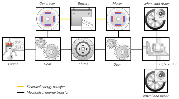
3. HEV reference

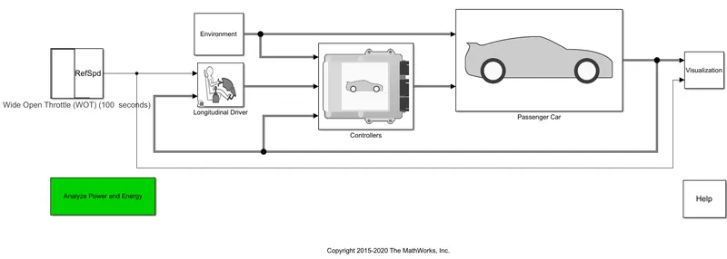
In the model setup, we have the Drive cycle input from the block Drive cycle source (link). Here we define the WOT parameters such as WOT start time, initial & nominal reference velocity, etc. The units for the velocity are also defined below. These values are specified in the block parameters.

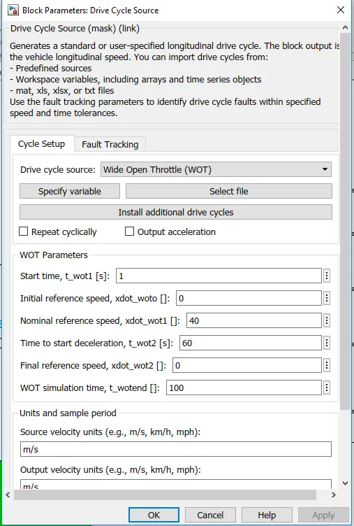
We give the start time for WOT simulation from 1 second. The initial velocity from where the WOT simulation is carried out is from 0. The nominal velocity is 40 and the time to start deceleration is 60. The final velocity after deceleration is 0 and the total time for WOT simulation is 100 seconds.

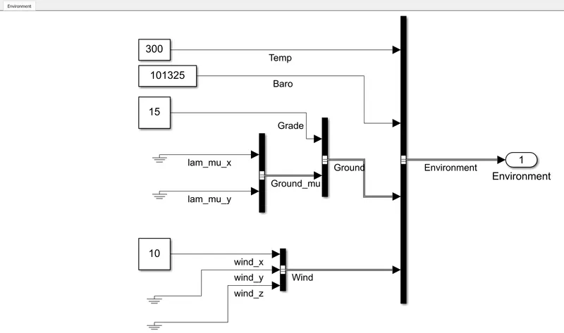
In addition to this, we also add the gradient value and the wind velocity acting on the vehicle. These are given inside the Environment block.

4. EV reference

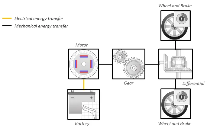
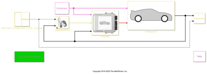
In the model setup, we have the Drive cycle input from the block Drive cycle source (link). Here we define the WOT parameters such as WOT start time, initial & nominal reference velocity, etc. The units for the velocity are also defined below. These values are specified in the block parameters.

We give the start time for WOT simulation from 1 second. The initial velocity from where the WOT simulation is carried out is from 0. The nominal velocity is 40 and the time to start deceleration is 60. The final velocity after deceleration is 0 and the total time for WOT simulation is 100 seconds.

In addition to this, we also add the gradient value and the wind velocity acting on the vehicle. These are given inside the Environment block.

EXPLANATION:

1.

Mapped model:

The mapped model refers to the block where the inputs & outputs of the block are given in steady-state lookup tables. For example, in the case of a SI engine block, the inputs of the engine like fuel intake quantity, air intake, etc. and outputs of the engine such as torque output, power output, etc. are given in the form of lookup tables. Mapped model simulation is to be done when we have engine data. This type of simulation model is used for quasi steady-state simulations.

The mapped model is used for simulation to study the effect of a factor on the simulation in the system level. For example, we can use the mapped engine model to study the effect of valve timing, quantity of fuel injected/sprayed, etc. on the engine output parameters.

This is similar for the motor and generator models.

Dynamic model:

Dynamic model refers to one which breaks down a system or sub-system into its components. The output of these components combined is taken as the output of the system. This type of model can be used when we need a more detailed model. To use this type of model, we need to have the component level data as we will need to give input to each of the componenets and take their output. This type of model is used to analyze the impact of individual components on the overall performance.

This is similar for the motor and generator models.

Changing b/w Mapped & Dynamic model:

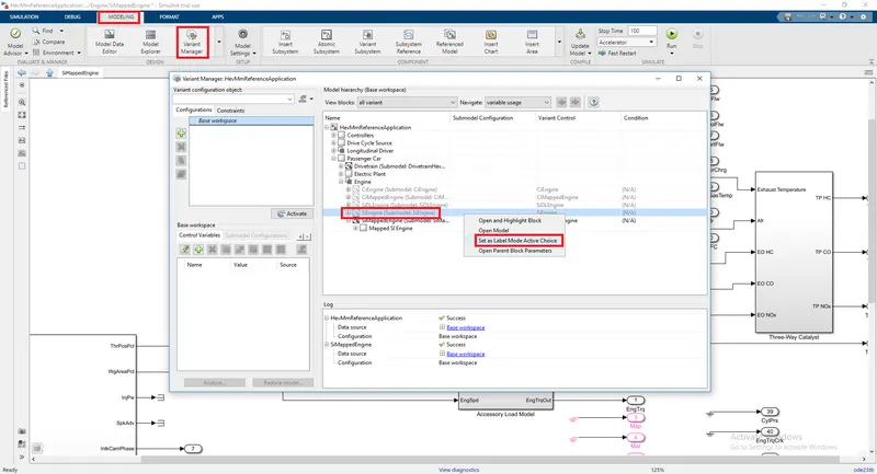
• Inside the Passenger car block, select the Engine block / Electric plant block / Drivetrain block.
• Open the Variant manager window from the Modelling tab.
• Select the desired type of model, right-click and select "Label mode active choice".

2.

For HEVs, the miles per Gallon is calculated by combining the fuel efficiency of the gasoline along with the electric power. It has been found that 1 gallon of gasoline is equivalent to 33.7 kWh of electrical power. This value is tested and given by the United States Environmental Protection Agency (USEPA).

For example, a battery propels the vehicle for 5 kWh capacity of battery, the miles per gallon equivalent is given by

5 miles/kWh *33.7 kwH/gallon = 168.5 mpGe

The miles per gallon calculation is done by the Performance calculations block (sub-system).

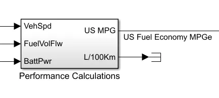
For this, the vehicle speed, fuel volume flow and the battery power is required. The distance travelled is calculated by integrating the vehicle speed with respect to time. Then the value is converted from m to mile. Fuel volume flow is calculated by integrating it similarly with respect to time. Along with this, the battery power is converted to kW and then converted to kWh/USgallon by dividing the obtained by 33.7. This value is then converted from `m^3` to US gallon. The two values are divided with each other and the miles per gallon value is obtained.

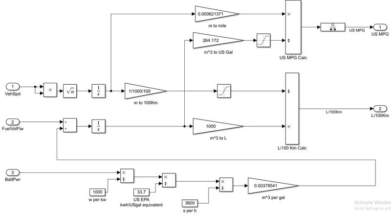
The factors considered for modelling fuel flow are Vehicle speed, Fuel volume flow and Battery power.

3.

Once the simulation is done, we will obtain the results in the form of plots. These plots can be obtained from the Visualization block in the Performance and FE scope.

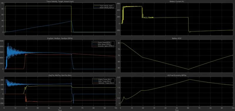
For the WOT condition, we can see the Trace and actual velocity in the first plot. The blue line represents the velocity that we had defined. The orange line represents the actual velocity. We can see that there is significant difference between the two curves. As the time increases, the actual velocity gradually increases due to gradient and wind forces acting on the vehicle. Also in the deceleration, we can see that the final velocity is 0 is obtained after the specified time which is 60 seconds. In terms of the Battery State of Charge, we can see that the SOC is constant at 80 for 1 second i.e. before the start of the WOT condition. From the next second, the SOC has reduced steeply to below 60. After 60 seconds, i.e. after the deceleration has started, we can see that the SOC increases again. For the motor speed, it is increasing from the beginning and after 30 seconds, it almost becomes constant at 5800 rpm. As the deceleration starts, the motor speed reduces to almost zero. The generator speeds is zero till the 17 or 18th second and after that the value increases. As the deceleration starts, the speed of the generator also decreases from around 5800 rpm to around 4200 rpm. As for the fuel economy, there is an increase in the fuel economy till the deceleration is about to start. After 1 or 2 seconds have passed after the deceleration has started, the fuel economy also starts to decrease. The battery current increases from zero to around 450 A and is almost same till 17 18 seconds. Then there is a dip to around 190 A and then till the deceleration starts, the value is same. After the deceleration has started, the current goes down below zero and then it becomes constant.

4. Comparing the HEV with EV, we get the plot outputs as follows.

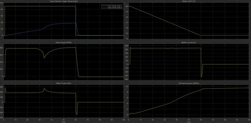
For the EV reference, we can see that the actual velocity curve differs from that of the HEV reference. Upto 33 seconds, we can see that the velocity increases at a particular inclination. Then when the motor torque has a peak value, we see that the velocity started to increase at a different rate. At around 32 33 seconds, we can see that there is the peak value of motor torque and there is a significant dip in the motor speed value. As the deceleration starts, there is a sudden decrease of the motor speed from around 4000. Similarly, the motor torque value also sees a sudden decrease as the deceleration starts. The torque value also goes negative and after a few seconds, the value becomes zero. For the battery state of charge, from the 2nd second, there is a steeper decrease than that for the HEV reference. However, the SOC value does not go below 74.5. As the deceleration starts, there is a slight increase and then the SOC becomes constant. The battery current sees a sudden increase from the start of the WOT condition from zero to around 210 A. It then remains constant and there is a sudden decrease as the deceleration starts. Further the value becomes zero after a few seconds.

CONCLUSION:

Thus all the difference between Mapped & Dynamic models is learnt, the simulation and comparing of the outputs of HEV and EV reference is done in the above project.