Week - 4 - 2D meshing for Plastic components

Objective

For the given Plastic Bottle Cap model, check for the geometrical errors and take the mid surface by suitable mid surfacing techniques. PID and Thickness assignment has to be done for all the mid surfaces.

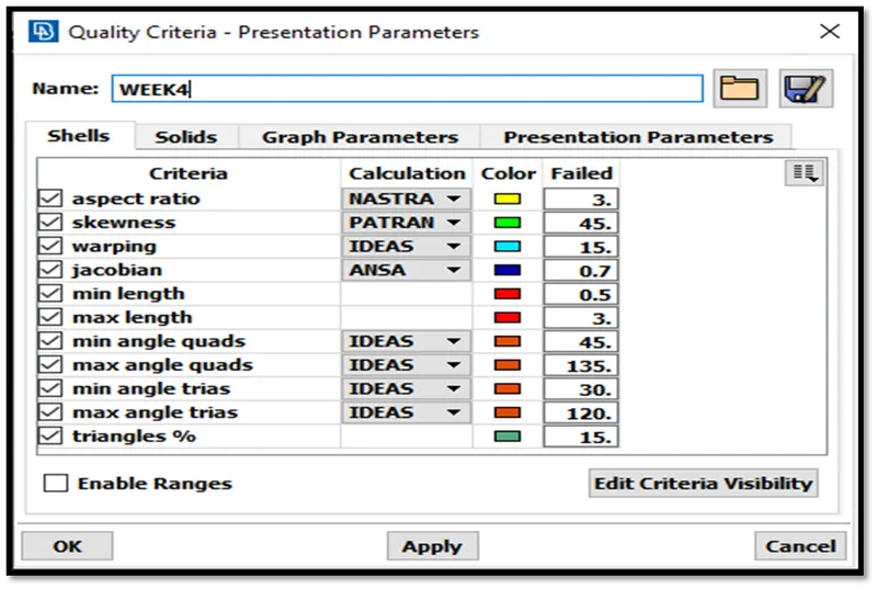
Mesh the same with given element Quality criteria. (Refer the table below for the Quality criteria)

Quality criteria

1. Target/Average length – 1 7. Jacobian – 0.7

2. Minimum length – 0.5 8. Minimum Quad angle - 45

3. Maximum length – 3 9. Maximum Quad angle - 135

4. Aspect – 3 10. Minimum Tria angle - 30

5. Warpage – 15 11. Maximum Tria Angle - 120

6. Skewness – 45 12. Tria Percentage – 15

Theory

The whole analysis domain has been divided in three major categories-

1. Pre-processing Solving 2.Solving 3. Post-processing

1. Pre-processing –It is also called meshing which is the first step in solving a problem in Finite Element Analysis. Here the entire domain in discretized (divided) into meaningful divisions often called "Elements". These elements form the building block on which the Boundary conditions and external effects are specified. The software used are ANSA & Hypermesh.

2. Solving – Evaluating the requirements of the product by applying boundary conditions. It doesn’t require much work as the whole setup comprises of partial differential equations and ordinary differential equations which are further integrated for the final results. All of these evaluations is done by software’s like – Ansys Workbench, Radioss, Nastran etc.

3. Post- processing - You can evaluate the results once the simulation has been completed and the displacements, stresses, or other fundamental variables have been calculated. The evaluation is generally done interactively using the Visualization moduleof CAE. The Visualization module, which reads the neutral binary output database file, has a variety of options for displaying the results, including colour contour plots, animations, deformed shape plots, and X–Y For ex- Meta-post, HyperView

Meshing a domain would consist of the following tasks

1. Defining a domain to Mesh

1.1 Importing a CAD Geometry (Computer Aided Geometry) OR.

1.2 Creating your own Geometry OR.

1.3 Creating node-based elements.

2. Selecting the analysis type (Ex: 3-Dimensional, 2-Dimensional, 1Dimensional).
3. Creating the mesh.
4. Choosing the element type.
5. Validating the mesh. Check for Errors, Connectivity, Quality etc.

Importing CAD Geometry

CAD standing for Computer Aided Geometry. It is a procedure of generating Virtual parts using Computers. It dates back to (almost) the beginning of computers.

In 1960s when digitizing Drawings, Surfaces, Generating Numeric Codes for automatic machining of metals gained popularity. As Finite Element Analysis became popular during the 1970s, meshing Native CAD geometry got importance.

Today much native CAD geometry can be imported into meshing software for the purpose of creating a finite element mesh. There are many neutral geometry formats available such as the popular IGES (Inter Graphical Exchange Specification)

Some of the CAD geometries that could be imported and meshed in commonly used meshers (Not exhaustive list..) are;

1. Pro-Engineer/Creo
2. CATIA
3. STL (Stereo Lithography Format Tessellation)
4. IGES (Initial Graphics Exchange Specification)
5. DXF (Data Exchange Format)
6. Parasolid
7. Unigraphics
8. ACIS (Andy Charles Ians System solid modelling geometric engine) etc.

Steps in Meshing

1. The first step in meshing would be to select a suitable element to mesh your domain.
2. Let's continue by saying that you have selected a 2Dimensional mesh of 1st order (corner nodes only) mixed mesh containing rectangles and triangles.
3. You could then define an element as the element type that you want to fill the nodes with (say trias) as follows

3.1 Example with trias: <element no>, <connecting node 1>, <connecting node 2>, <connecting node 3>

3.2 Example with quads/rectangles: <element no>, <connecting node1>, <connecting node 2>, <connecting node 3>, <connecting node 4>.

Node

Nodes form the building block of any mesh. An element is specified through its connectivity to a set of nodes. Nodes can be simply thought of as a coordinate which has a label to it.

So that when you refer to this label, you mean the coordinate. A sample node may look like this.

Node Label 1, X Coordinate, Y Coordinate, Z Coordinate

Notes: Node has to be defined according to the Coordinate system to which it refers. (In majority of the solvers the default would refer to a Global Cartesian Coordinate System)

Most of the example defined may refer to ANSA and hyper mesh software. But an attempt to generalize the examples is also on.

Element Quality

Element quality is very important for a solver to provide you with a reasonable result.

Element quality is most often defined as a deviation from a perfect element.

It's important for the user to understand what is Iso-Parametric element &

Order of element. An element can be of either 1st order or 2^nd order.

Elements can be classified into many kinds, but the most important classification would be; Structural and Continuum.

Some of the basic element quality checks;

Element Quality Criteria

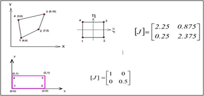
1. Jacobian - The Jacobian ratio is a measure of the deviation of a given element from an ideally shaped element. The Jacobian value ranges from -1.0 to 0, where 1.0 represents a perfectly shaped element. The ideal shape for an element depends on the element type. The check is performed by mapping an ideal element in parametric coordinates onto the actual element defined in global coordinates.

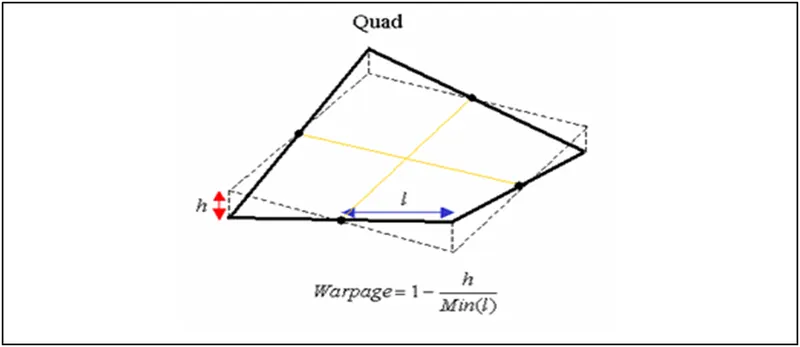
2. Warpage - It is defined as angle between normals to two planes formed by splitting the quad element along diagonals. Max. angle out of the two possibilities is reported as warp angle. You can also say it as, in any quad element one node out of four is out of plane.

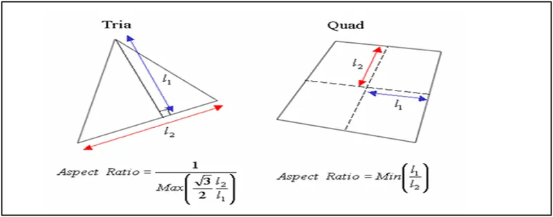
3. Aspect Ratio - Aspect ratio is the ratio of Maximum edge length to the minimum edge length of an element. The ideal value of aspect ratio is 1. That means all the sides of an element are of equal length. However, an aspect ratio of less than 5 is generally accepted. If aspect ratio is greater than 5, it means that max length is 5 times greater than min. length of the element and the element is said to be failed in aspect ratio criteria.

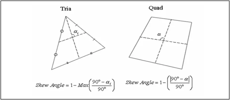
3. Skew - An angle is formed by the two lines which pass through the midpoints of the sides of the quadrilateral. The skew angle represents the absolute value of the difference between the angle and 90 degree. A rectangle has the skew angle of 0 since the formed angle between lines is 90 degree. For the triangle and quadrilateral elements, the skew angle is found as shown in the figure. For solid element (Tetra, Hexa, Wedge), it calculates the skew angle for each element faces and assigns with the minimum value.

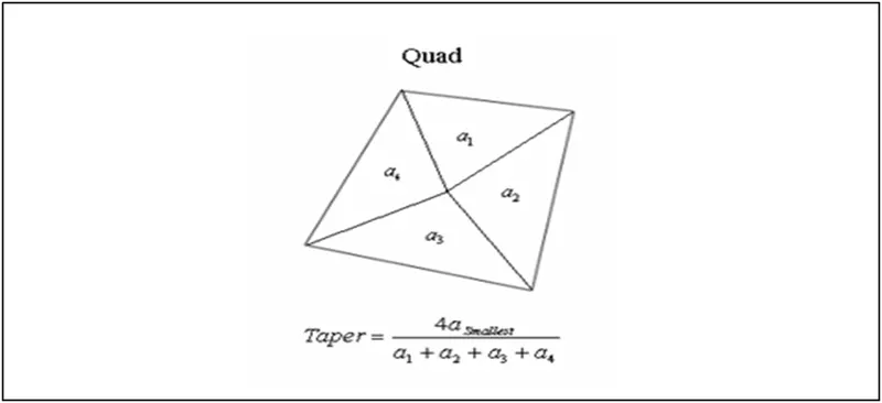
4. Taper - It checks for the amount of deviation of the quadrilateral element from a rectangular shape. A rectangular element has the taper of 1, and it gets away from the rectangular shape (closer to the triangular shape), the taper becomes smaller. For the quadrilateral elements, the skew angle is found as shown in the figure. For solid element (Hexa, Wedge), it calculates the skew angle for each element faces and assigns with the minimum value.

5. Minimum length - The Min Edge Length value determines the minimum edge length of a mesh cell.

6. Maximum length - The Max Edge Length will be limited to 24% of its specified value. Maintaining the specified Min Edge Length will result in an effective Max Aspect Ratio of 2.5.

For our project we will be using ANSA for whole objective.

Why ANSA?

ANSA (Automatic net generation for structural analysis) ANSA is a computer-aided engineering tool for Finite Element Analysis and CFD Analysis widely used in the automotive industry.

It is developed by BETA CAE Systems. The software is distributed worldwide by a number of BETA CAE Systems subsidiaries and business agents. In the United States, it is distributed by Beta CAE Systems, USA, based in Farmington Hills, Michigan.

ANSA maintains the association between CAD geometry and the FE mesh. This means that the FE meshes are better representations of their geometric parents.

Also, it is easy to maintain and update any changes in the geometry by simply reworking the updated area instead of recreating the FE from scratch.

It carries several proprietary algorithms for meshing suitable for both CFD and structural models.

Procedure

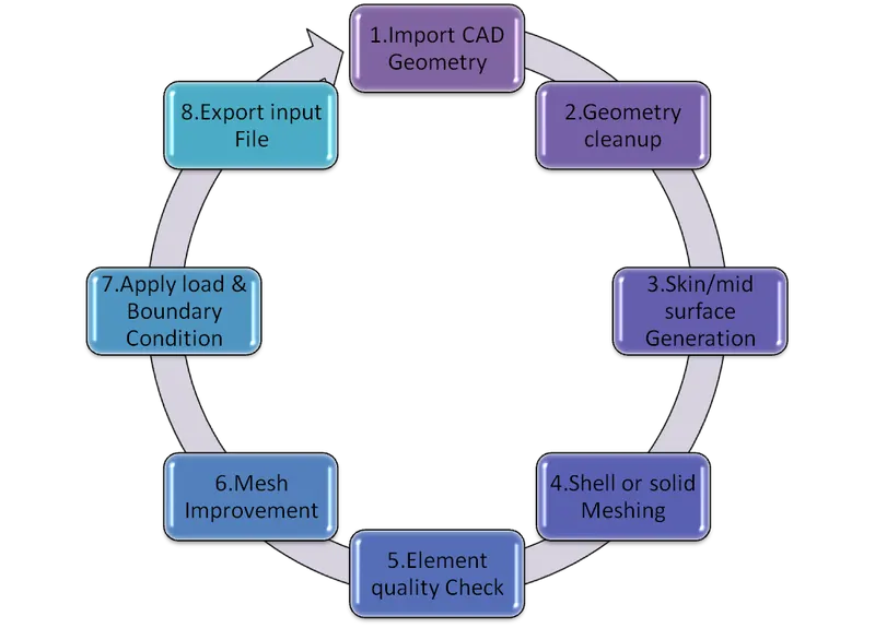
There are various steps in meshing and mid surface generation as shown in flowchart.

Our job is to only create mid surface and improved mesh for the particular component.

The provided component is a hood of car, which is being manufactured from sheet metal. We will be using 2D or shell meshing for the sheet metal component as the two of the dimensions is quite big as compared to the third one.

X & Y >>>Z or length & Breadth >>> Thickness

Importing CAD Geometry

*Download the CAD model from dashboard

*Open it using path File>open

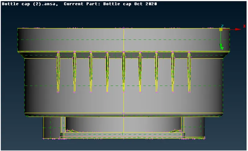
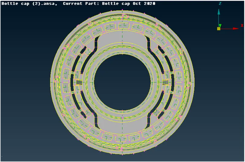
FRONT VIEW OF THE BOTTLE CAP

BOTTOM VIEW OF BOTTLE CAP

GEOMETRY CLEANUP

Cleaning a geometry means taking out every possible error in the geometry which can affect mesh generation and finite element model. These are some listed errors which must be checked before meshing-

Single cons – The boundaries of a surface represent single cons when they are not connected with any faces. The red lines showcase single cons in geometry. We need to check for those single cons who are connected with faces but showing as single cons.

Double cons–When an edge of a face is shared between two or more faces it is called double cons. It is shown as yellow lines in the geometry. We need to check for those edges which are single cons but it is showing yellow cons or triple cons as an error.

Triple cons – When the edge of a face is being shared by three or more than three faces it shows triple cons. These types of cons are present more in mould and casting.

It is shown as cyan lines in the geometry. We must check for those cons which are double cons but showing triple cons.

Cracks – These are the areas which are not joined systematically by any con system. Hence in most of the cases it is shown as single cons which are needed to be joined to make the geometry crack free or

sometimes the hotpoint or node which is used to connect cons are missing.

Overlap Faces – The faces which have an extra area or the duplicate faces which overlaps one of the faces are called overlapping faces. We need to rectify these faces as they consist extra nodes, hotpoints and cons, which leads to error increment in the solution.

Needle Faces – The faces which are compromised for fillets, beads or other features were the area of the face is very less like a needle which creates a confusing situation for ANSA to treat it like a face or a con.

Collapsed cons – These are the cons which are accidentally formed in conversion of the part file. They are mostly extra cons with a convergence towards any edge.

Command used in clean-up

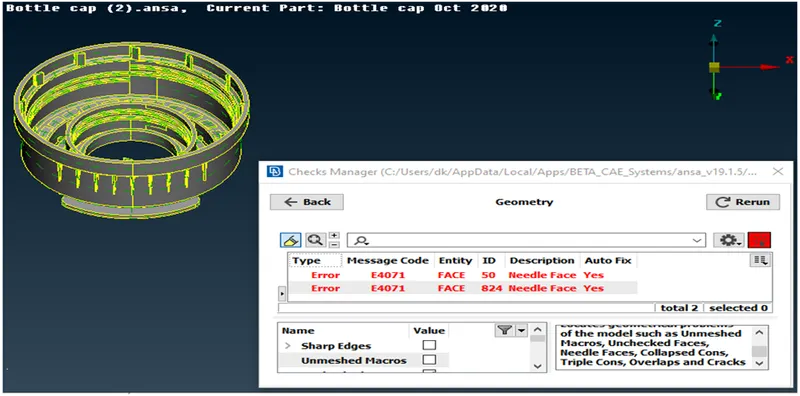
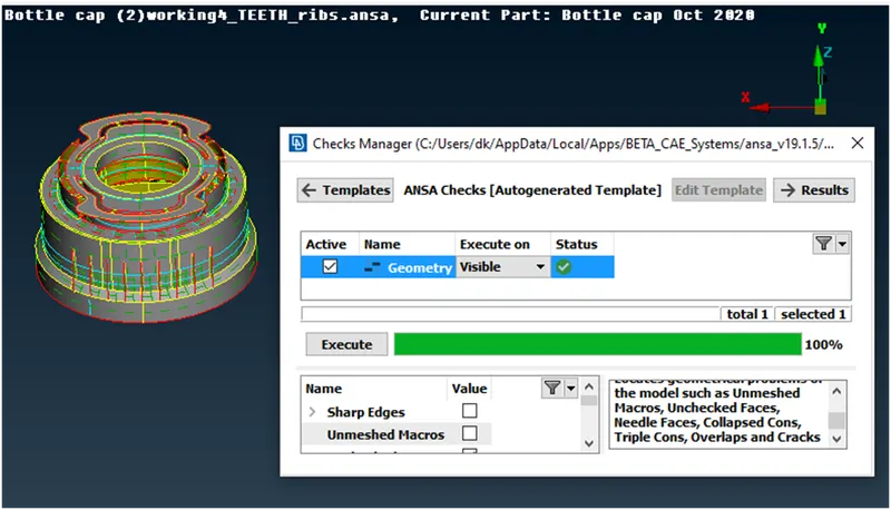
*Check – ANSA have a strong algorithm to find all listed errors, within a short range of time and classifying in its proper class. The ability to find errors provides ANSA a nice capability to fix basic errors by its own by using autofix option.

Syntax line to check geometry-

Tools >check >Geometry>Execute

Geometry check and listed errors

Syntax line to Autofix-

Select all > Right click > Fix

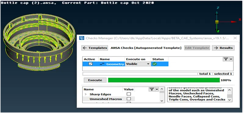
If sometimes auto fix doesn’t work we switch to manual mode. Which involves releasing of the unwanted cons sometimes deleting and performing topology?

Geometry check and errors fixed

Orienting faces

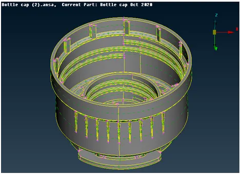
The geometry should be aligned to the referenced body parts so they are categorized in negative & positive sides.

ANSA do provide options for manual and automatic orienting according to the amount of positive and negative side

Syntax line to orient geometry

Select faces > orient > Middle mouse button

Orient > Select > faces > Middle mouse button

Orient > Visible

For selections of faces we need to activate cross hair selection for individual face selection. For applying the command, we can press enter or Middle mouse button.

Positive side

Negative side

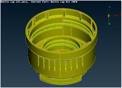
Mid Surface Generation

The midsurface modelling process relies on an accurate solid model as the starting point. Midsurface modelling is best suited to thin solids or thin-walled solids where wall thickness is constant or

where reasonable approximations of the wall thickness at each point can be made easily. You can apply midsurface modelling to any solid cell within a model; you need not apply it to the entire model. If you apply midsurface modelling to only a portion of a solid model, Abaqus/CAE automatically creates shell-to-solid coupling constraints to couple the motion of the midsurface shell edges to that of the remaining solid model faces. Shell-to-solid coupling constraints will not be created if the angle between the shell surface and the solid face deviates significantly from 90°.

Besides reduced expense, you might use a midsurface model in place of a solid model to better account for bending response in thin sections of the model. Shell elements are designed to manage bending loads within the thickness of a single element, whereas a single solid element will have little or no resistance to bending.

The provided model has different types of component as listed

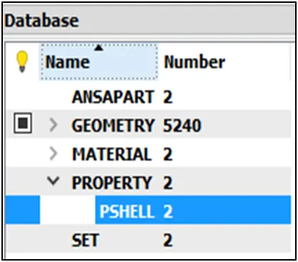
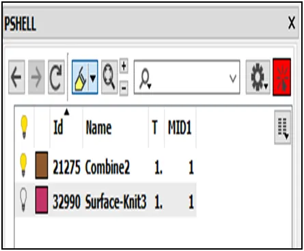
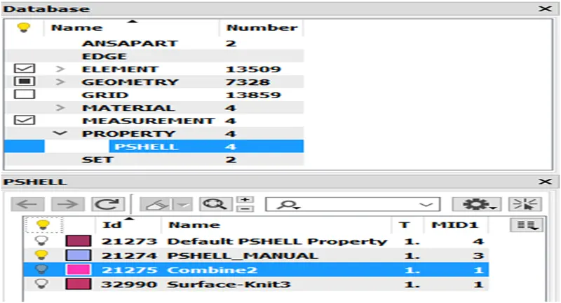
Database – It is basically the data storage which consists of everything which the model is comprised of like part numbers, Geometry type, Material and individual property ids called PSHELL.

These individual PSHELL are the separate parts formed in single operation or does share some similarity. They are listed as Default shell property and specified color which can be seen separately using show only.

So there are 5 parts and have individual separate property ids, so the midsurface generation of all these parts will have their own ids with specified thickness.

ANSA provide options for manual and automatic mid surface generation

Command used in mid surface generation

Measure – This command is used to measure distance between nodes, cons & faces and also enable us to save the measurement in store which is shown in database.

The reason behind measuring the thickness is to get the thickness value and provide the exact half while generating mid surface.

Offset – This option is mainly used in manual midsurfacing, the faces are selected and exact half value is provided with proper orientation to get it in between the parts.

OR – It is a selection tool, which works with cons and faces. It brings out the selected region separately and rest of component becomes hidden.

NOT – This tool help the user to hide the region when selected. It is just the opposite of OR.

AND- This tool enables the user to bring out neighboring region which has been selected with help of OR & NOT.

!NOT – This is hybrid tool selection option. We can select any region and press middle mouse button, that part is isolated from rest of the component.

ALL – This command help the user bring out the entire hidden component at once.

INVERT - The region or part which we select with help of selection tools shows in an different view. To change the view between the selected part and rest of the component the invert option is used.

LOCK- It is view storing option, which helps us to store views and also the selected regions in inverted selection. It can be used in multiple ways it also get stored separately in database. It can be used as AND by using Neighboring > 1^st level.

This brings out the entire region which is connected to the selected region. It can be also used as ALL command by using Neighboring > ALL.

FINE – This option enable us to simplify geometry which get affected due to resolution issue.

FACE > NEW > FITTED – This option enable us to create new faces with suitable boundary conditions.

PASTE – This option helps us to face one con on another .

CURVE>MIDDLE – This command help us to create a middle curve between two cons.

TRANSFORM>ROTATE – This command help us to copy multiple entity as well as rotating all the entities at a certain angle with respect to two centre points.

POINTS>ONCOG- This command help us to create a 3d centre of the body or the part.

FACES>EXTEND – This command extends a edge having single con to the selected face.

CURVE>CONS2CURVE – This command converts cons to curve without changing the actual curve.

Syntax for Mid surface

Utilities > Measure > Nodes > Middle mouse button > Store

Offset > Feature > offset value > Middle mouse button

This process of midsurfacing is easy and automatic and also takes less time all these mid surfaces should be checked for geometry errors like triple cons and orientation and it should be rectified before proceeding to meshing.

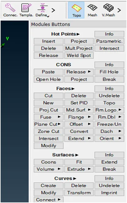
After creating the midsurface we need to find out extra cons and hot points which can effect in mesh generation. We should clean geometry on that basis.

Commands used for midsurface cleaning

CUT – This command help the user to deactivate the cons at the edges were mesh boundaries are formed.

DELETE – This command help the user to delete extra hotpoints which can affect the shape of the elements.

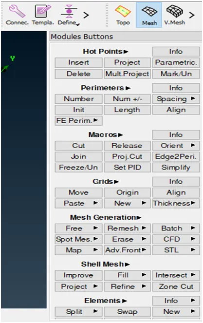
This is the listed toolbar for TOPOLOGY and MESH

TOPOLOGY MESH

To find errors we must carefully observe all the improper cons & hotpoints so that they can be deactivated.

NOTE – Fillets are key features as they provide curvature to the face and their forming cons mostly double cons should be considered with proper care so that elements can have least distortion in covering the geometry.

Meshing

A mesh is a network that is formed of cells and points. It can have almost any shape in any size and is used to solve Partial Differential Equations. Each cell of the mesh represents an individual solution of the equation which, when combined for the whole network, results in a solution for the entire mesh.

Solving the entire object without dividing it into smaller pieces can be impossible because of the complexity that is within the object. Holes, corners and angles can make it extremely difficult for solvers to obtain a solution.

Small cells, on the other hand, are comparably easy to solve and therefore the preferred strategy.

Mesh Types

It’s common to classify mesh types as structured (curvilinear) or unstructured. As discussed before, structured meshes are historically related to the Finite Differences Method. The Finite Volume and Finite Element methods allow for more general meshes.

Structured Meshes

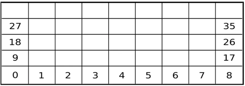
Structured meshes, also commonly called grids, are meshes whose structure and formation allow for easy identification of neighbouring cells and points. This property is derived from the fact that structured meshes are applied over analytical coordinates systems (rectangular, elliptical, spherical, etc.), forming a regular grid.

Unstructured Meshes

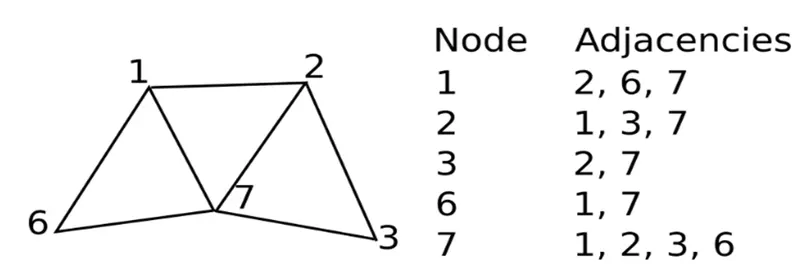
Unstructured meshes are more general and can arbitrarily approximate any geometry shape. In contrast with structured meshes, where the coordinates and connectivity’s map into the elements of a matrix, unstructured meshes require special data structures,

such as an adjacency matrix or list and the node coordinates list. The unstructured mesh node/cell numbering can be arbitrary and sparse since it does not require any analytical form of adjacency query.

Commands used in mesh generation

INSERT – This option hep the user to insert hotpoints so that cons can be formed or faces can be joined.

NUMBER – When there are odd numbers of hotpoints in a particular feature or hole, they are checked by using this option to convert it in even numbers.

MARK/UN – The converted feature from odd to even is marked up, so that it doesn’t get back to its original state.

NUM +/- - To add or subtract hotpoints from a feature or face we used this option.

CUT – This option helps the user to divide the component in several parts, so that best possible meshing can be generated in smaller areas.

RELEASE – As we know every con or hotpoint is connected to adjacent cons & hotpoints, so if we want to change or delete any one of them we must release it dependencies on other feature.

JOIN – It’s the opposite of cut, it help the user to join part by different means by keeping the mesh same or reconstructing it while joining.

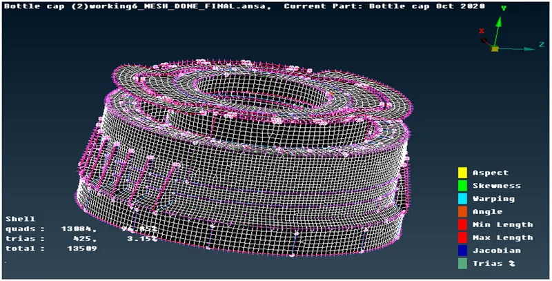
SET PID – For every new midsurface we must assign a separate property id,thickness, material and color, so that they can be classified as separate PIDs.

BEST – To create a mesh in the specified area which is being divided with help of cut command this command is used as it tries to create mesh as best as possible.

RECONSTRUCT – To reconstruct a best mesh to fit within quality criteria sometimes it’s needed to reconstruct it according to the boundaries.

SMOOTH- It smoothens up the mesh lines so that it can fix quality issues.

SWAP- It just swaps the element length to adjacent node. It is used to adjust element and eliminate trias as more as possible.

SPLIT- Sometimes it is required to divide the element to eliminate trias, split command is used for that purpose.

For different views and properties there are various tools

ENTITIES- It is the default settings in which we can observe different entity for further classification.

PID- These are property ids for components, which shows component for specified property and material.

SHADOW – This is a visualization option which helps us to observe the component in original cad form and meshed also.

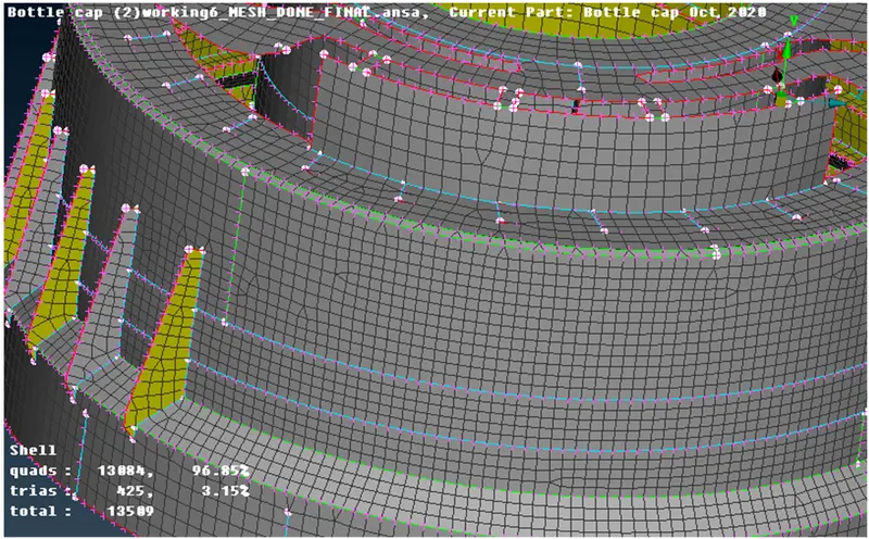
HIDDEN - This is a visualization option which helps us to observe the component in edge form. This option also shows hidden surface line and all cons present in the component. It also showcases the failed elements according to quality criteria.

This is the best possible view method to rectify failed element and adjust elements by using split and swap command. The cons are shown green in color and element as white grid.

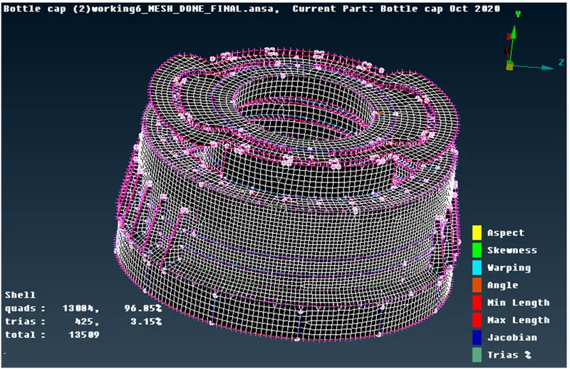
Mesh Quality – This option enable us to check the meshed component according to specified quality criteria. With the help of this option we can find out those elements who failed the criteria and needed to be reconstructed.

These are the listed components detail with quality checked

1. Meshed midsurface with quality checked

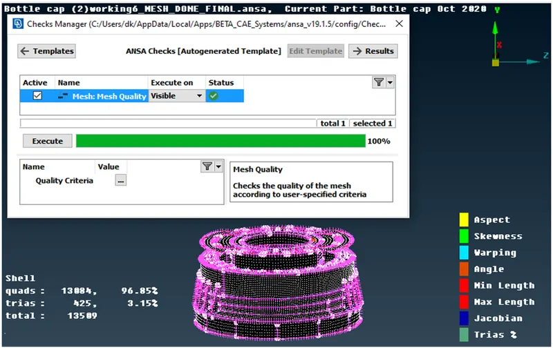
At last we need to release our fem model for the geometry to eliminate the associativity from the cad geometry.

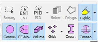
After releasing the fem model we can visualize the geometry and fem separately by using this listed option.

ASSIGNING THICKNESS: - By using Set PID in macros in mesh domain,we have to assign thickness of each individual midsurface.

MESH > MACROS >SET PID

SELECT FACES>MIDDLE MOUSE>RIGHT CLICK>NEW>P SHELL

ASSIGN THICKNESS >DOUBLE CLICK ON PSHELL

QUALITY CRITERIA> DRAW SHELL AS SOLIDS

Final image of the model

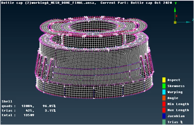
MIDSURFACE WITH MESH

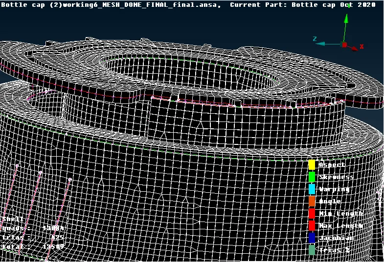
MESH DRAWN AS SOLIDS

Conclusion

The geometry cleanup is a key part of pre- processing and it affects a lot in shell meshing. The fillet feature is should be carefully observed and meshed.

There are some basic meshing rules to take care off

• No two trias should face each other.
• There should not be any trias immerging from the edges.
• Minimum number of trias should be preferred in the fem model.
• The number of nodes in hole features should be even.
• All elements should pass the quality criteria.

Google drive link for the model

https://drive.google.com/file/d/1ISNYE-fV4niabJaGKHM4g3f_38jPlMQW/view?usp=sharing