Transient simulation of flow over a throttle body

Aim:-

• Set the transient-state simulation for flow over throttle body case setup in the converge.
• Export all the input files and run the simulation using Cygwin.
• Converge plot for velocity, pressure, mass flow rate, and total cell count.
• create animations of velocity and pressure contours plot for the flow inside the elbow pipe in which the throttle movement should be visible.
• Show mesh (i.e surface with edges) by creating a mid surface/slice along the z-direction.
• Explain the plots and write a detailed report on the project.
• Create another animation in Paraview representing streamline flow over throttle with transient state simulation.

Objective:-

• Import the throttle geometry model in the converge using the create option.
• Perform Geometry cleanup.
• Define the boundary to each surface of the geometry.
• Set normal direction on the inward side of the surfaces. means, define the direction towards the volume where the fluid is present.
• In case of setup define the material, simulation parameters, fluid region, boundary condition, no of cycles, grid definition.
• Extract the setup files in the simulation folder.
• Run exported input setup files in Cygwin.
• Post-process all the results into 3D outputs and open in Paraview.
• Show mesh generation on the 2D mid surface by using the slice command from the Paraview.
• Plot converge plot for velocity, pressure, mass flow rate, and total cell count.
• Create animations in the Paraview to show the changes in velocity and pressure contour with the throttle movement
• Create other animations to show the streamlines of the flow over the throttle body.
• Explain the plot animations and write a detailed report on the project.

Modification of setup:-

For the transient Simulation, we just have to do a little modification in our previous steady-state simulation setup.

Simulation Setup/ Case setup:-

Application type:-

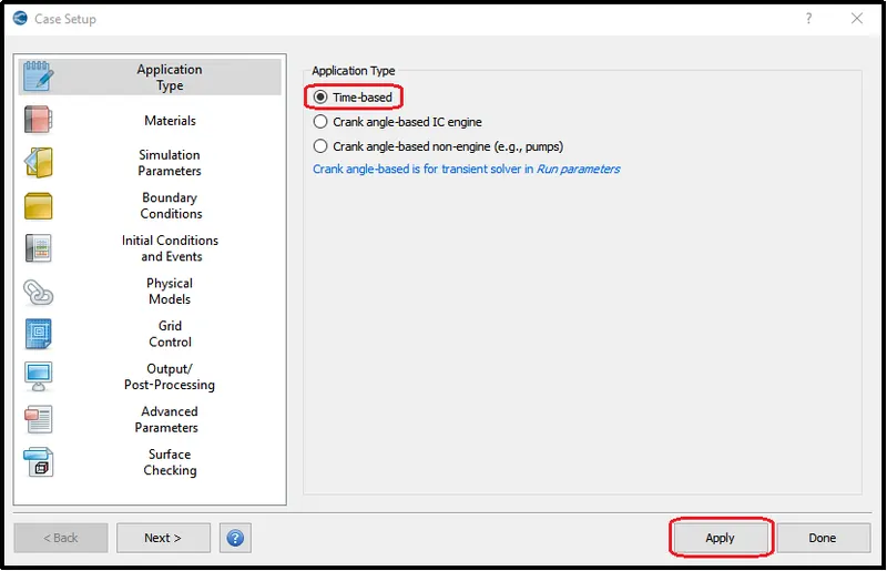
To begin with the transient state simulation in the 'Application Type" the "Time-based" must be selected and then, click apply and done.

Material Definition:-

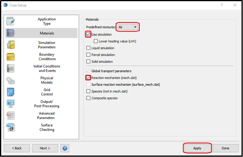
In this simulation, we simulated the results for compressible flow with fluid air.

Simulation Parameters:-

Run Parameters:-

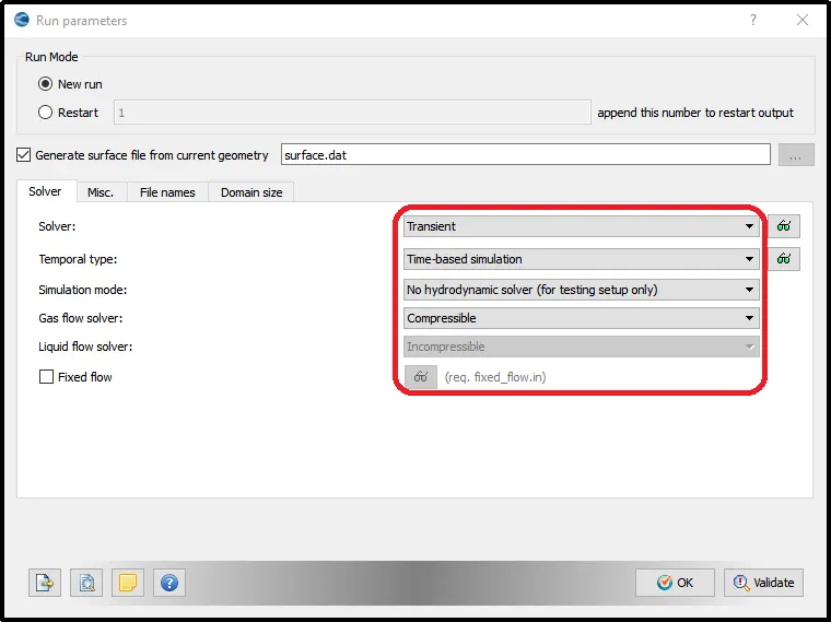
In the run parameter, we get to decide that either, we want steady-state simulation or Transient state simulation, so for the current simulation, the transient solver type was selected. This simulation involves the throttle movement which involves the changes in meshing while creating movement. To run this operation smoothly "NO hydrodynamic solver (for testing setup only)" option was chosen.

And, finally, as we are using air as a fluid that is compressible in nature so gas flow solver is set as compressible.

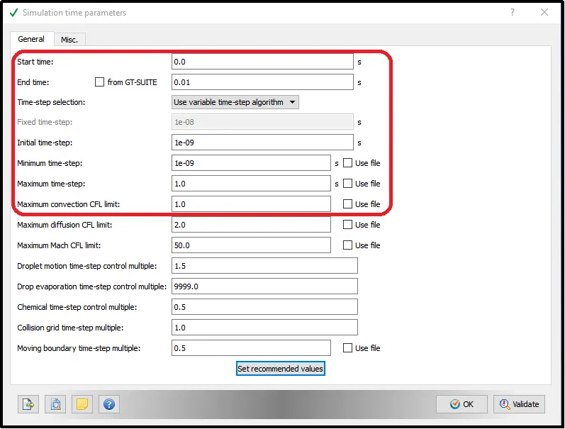
Simulation time parameters:-

For the transient simulation, we have to set the run time of the simulation. So for the run time calculation, we require the flow length and velocity.

`R u n T i m e = (F l o w L e n g h t) /(V e l o c i t y)`

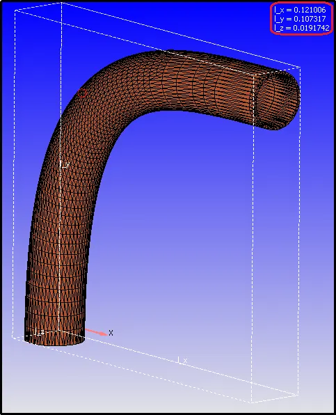
From the elbow, X-axis and Y-axis lets consider the maximum Flow length is 0.2m

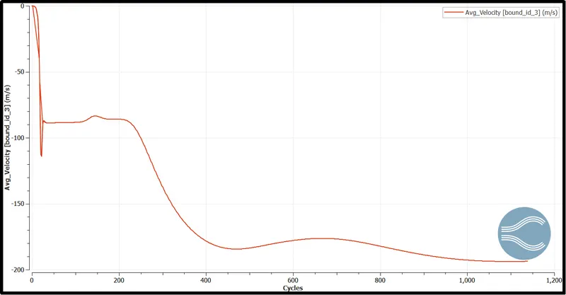
From our previous simulation, our average velocity inlet was 194m/s so as round figure take it as 200m/s

`R u n T i m e = 0.2/200`

`R u n T i m e = 0.001 sec`

Suppose we are going to simulate 10 times airflow from inlet to outlet.

Then, `R u n T i m e = 0.001/10`

Therefore, `R u n T i m e = 0.01 sec`

Fluid Region:-

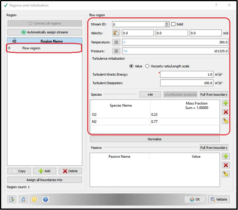
Apart from the boundary surface, cells also generate in the inner volume. Therefore, it is important to assign some material or fluid material with particular property conditions to these cells.

So, we define it as a flow region with material fluid as air with normal pressure and temperature at its initial state.

Boundary Conditions:-

Inlet:-

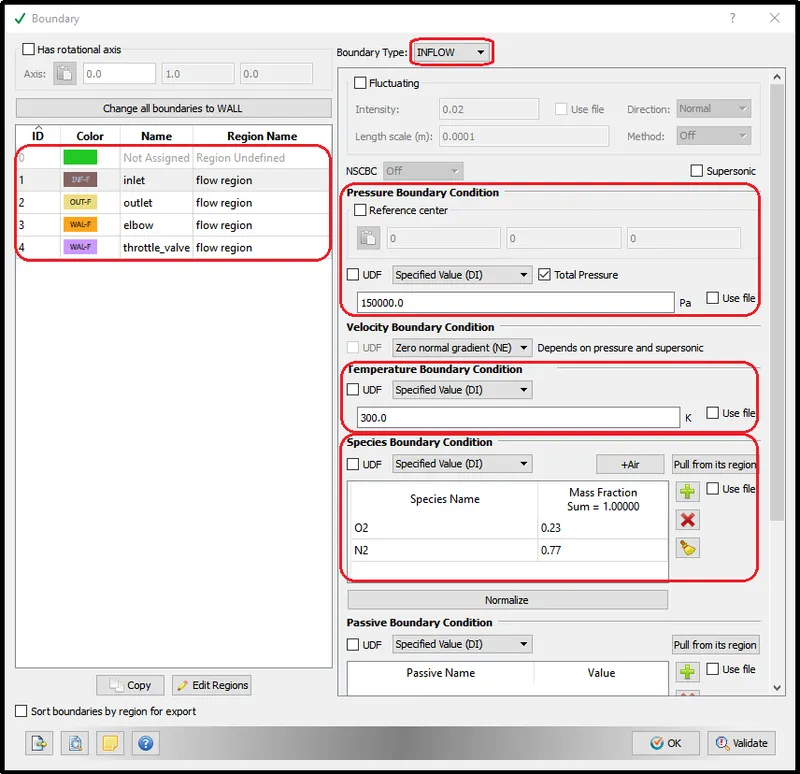
At the inlet, we are giving a pressure of 1.5 bar with a 300k temperature as an air inlet.

Outlet:-

At the outlet, normal atmospheric pressure and temperature conditions are considered.

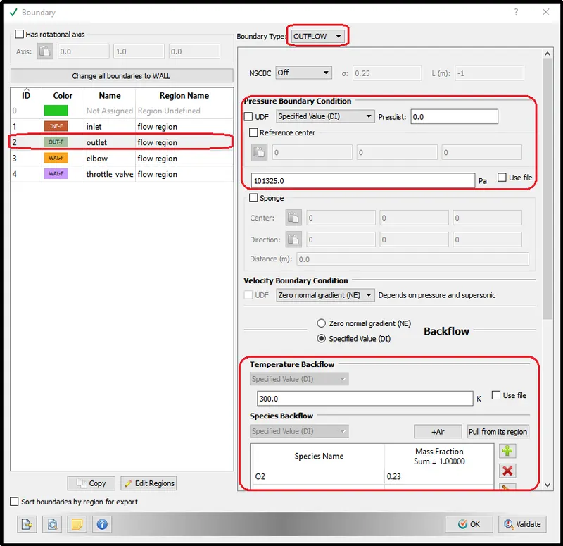
Elbow wall:-

The Elbow wall is the casing wall so it will be at stationary condition fixed surface. with normal law of wall condition.

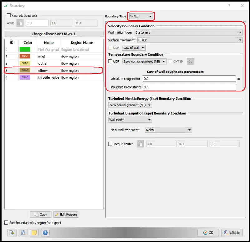
Thottle_valve:-

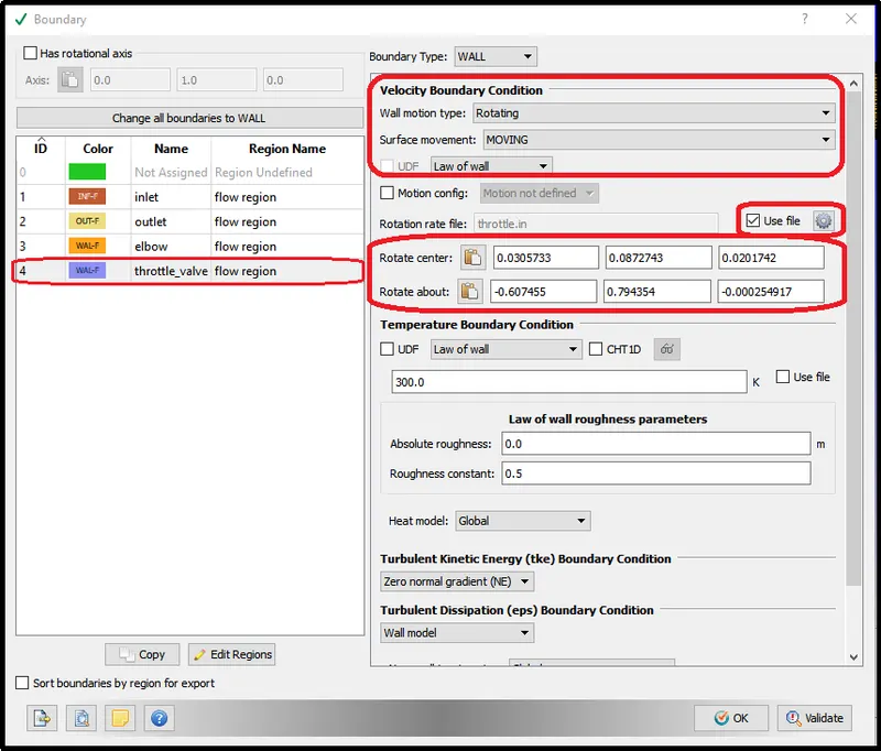
This time for the transient state condition the throttle valve was defined as rotating so the surface movement was also set as moving which following the Law of the wall.

the Rotation center was calculated using the measure tool and the value was copy and filled in the boxes. Same way, the rotation romal to that center was also calculated and copy-pasted in the blank box.

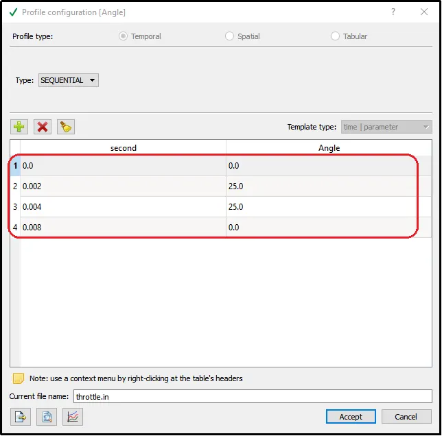
To give constraint motion to the throttle use the use file option and provide the rotation and time detail for the throttle movement.

After clicking the use file setting button below window will pop up. here the time and angle of rotation values of the throttle were provided to the throttle. form 0-0.002sec there will be no movement of the throttle. Then from 0.002-0.004sec the throttle rotates and maintains the angle of 25 degrees and after 0.004sec the throttle will rotate to its original position.

Turbulence model:-

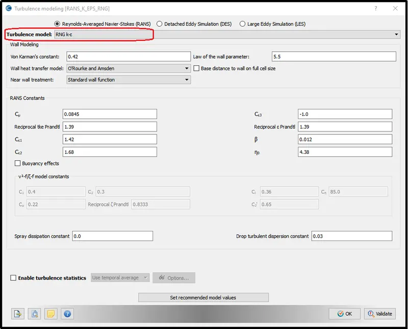
Here, the turbulence model was used as RNG K-epsilon. because because of obstacle or throttle valve the laminar stream converted into turbulent.

Grid Control/ Meshing:-

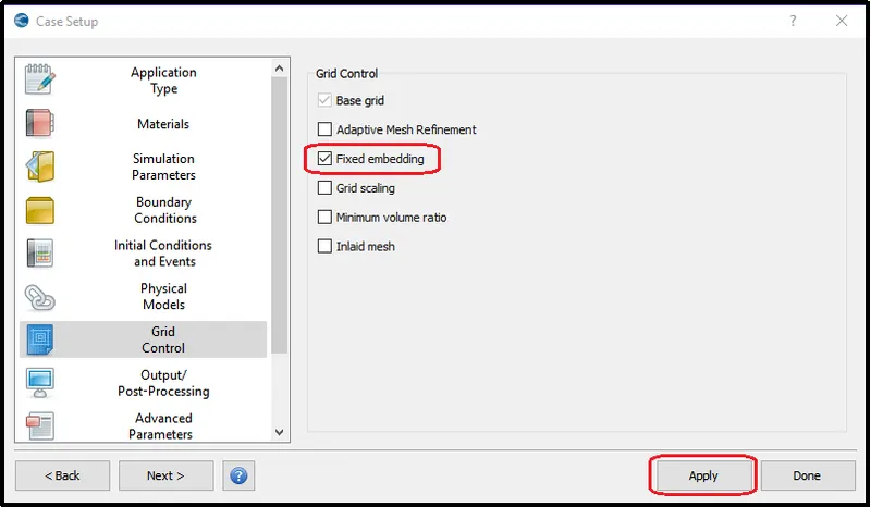
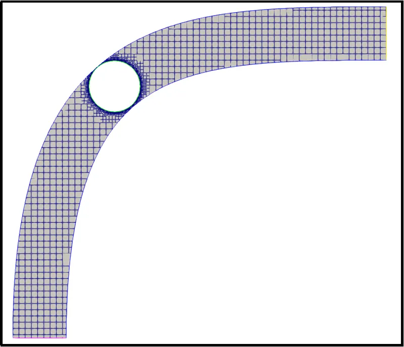
In the 'Grid Control' setting add the "fixed embedding" parameter.

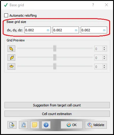
The grid size of 0.002m was given to all the directions.

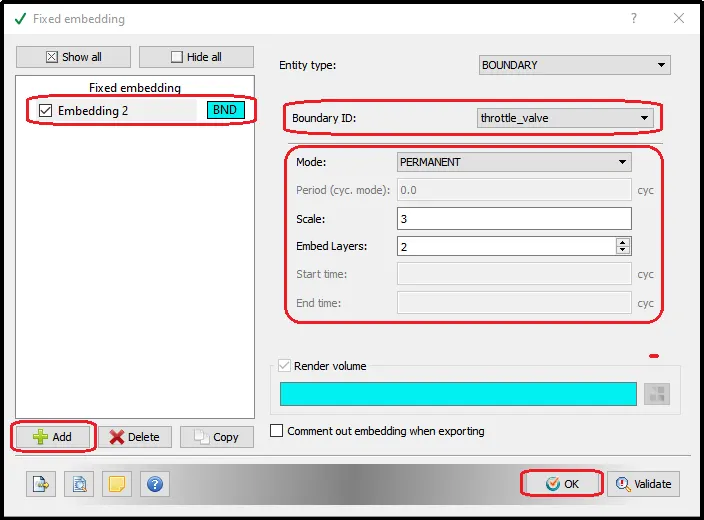
Near throttle wall surface fine mesh si required to capture accurate fluid flow near the throttle wall. The density of the cell near the throttle will give a clear representation of flow change near the throttle wall.

so the scale was used 3 with embedded layers of 2.

The mesh over the geometry looks like this after using the above setting parameters.

Output/Post-processing:-

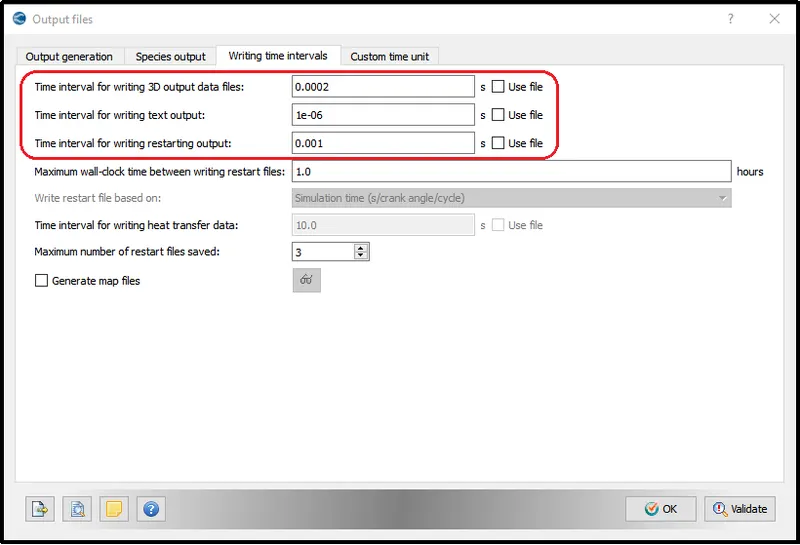
To get 3D output Time interval for writing 3D output was set to 0.0002sec means we are going to get 50 3D output files from this simulation.

The same calculation was used to get a time interval for text output data and a Time interval for waiting for restrating output files.

Complete Case setup:-

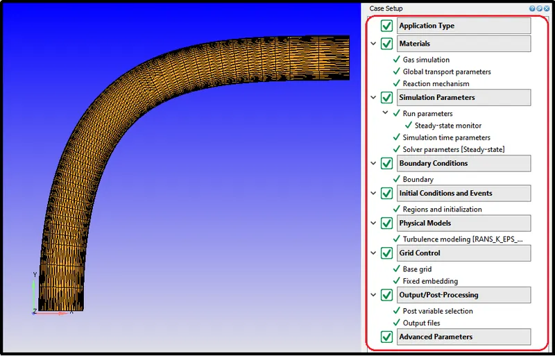
Converge shows a good representation of the completion of each case setting. It shows that the setup is correct by representing a green checkmark as portrayed in the below figure.

Export Input files:-

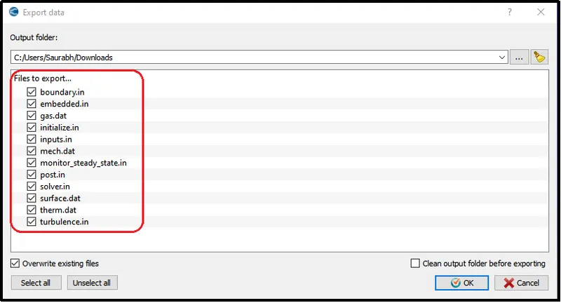
Using file -> Export -> Export Input files all the input files were exported to the simulation folder.

Simulation Run:-

The simulation was run with the help of Cygwin. The directory contains all the export files that were located and using the ‘converge.exe’ setup the simulation was run.

Convergence plots for Average Velocity at Outlet:-

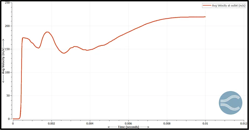
The following chart shows the changes in the velocity at the outlet of the elbow pipe in the simulation runtime span. at the initial state, there is no flow condition as the air gets time to flow from inlet to outlet. Then, we can notice the drastic rise in the velocity which shows the velocity suddenly appear at the outlet.

Afterward, the velocity starts to fluctuate which happens because of the throttle movement from 0.002sec to 0.004sec, and then it slowly starts to give us steady behavior as the throttle valve comes to its initial position.

Convergence plots for Pressure at outlet:-

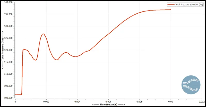
As we saw the velocity variation at the outlet, the below figure shows the pressure behavior with a change in time at the outlet of the elbow pipe. At the initial state, there is no movement then pressure shows a sudden rise as inlet air reaches the outlet.

Pressure also shows fluctuating behavior with the rotation of the throttle valve and when the throttle reaches its original position it starts to give steady results.

Convergence plots for Mass Flow rate at the Inlet and Outlet:-

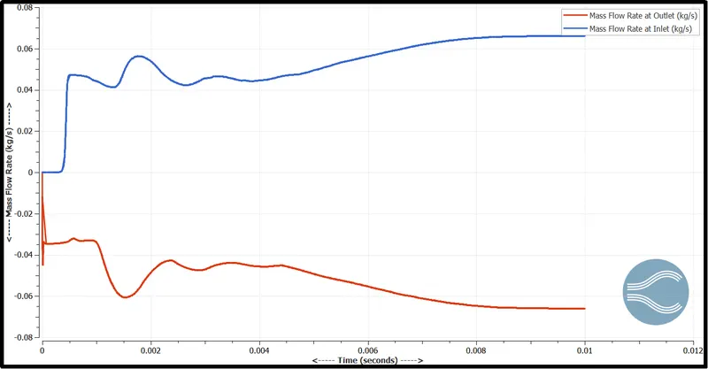
We can compare mass flow rate at inlet and outlet by taking look over the below line graph.

There is no movement at the outlet at the starting but at the inlet, we can notice the sudden rise of the mass as the inlet surface experiences sudden air velocity movement. The same movement we can observe for an outlet, as the air reaches the outlet surface, shows a sudden rise in mass flow rate in the outlet.

Then, the simulation solution follows the continuity equation as the mass flow is equal to mass flow out, where the line graph shows the inlet and outlet mass flow rates are almost similar.

Total cell count:-

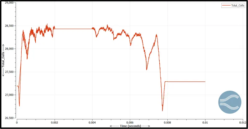
In transient simulation because of the throttle movement the total cell number change with respect to the throttle movement and time. Therefore, the following chart shows the fluctuation in the Total cell count in overall simulation time.

Velocity Contour:-

In transient state simulation, it is not good practice to observe simulation at a particular time or interval. Observation of total changes in parameters is an important factor. So the below video shows the velocity variation of the air with time and throttle movement.

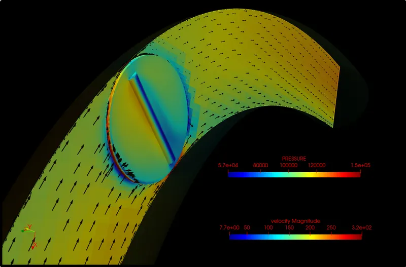
The velocity of the fluid (air) strikes on the valve body which is responsible for the high pressure on the front side of the body and at the back part because of less aerodynamic shape eddies form near the back surface of the valve. which is responsible for the lowest pressure on the valve body. To get closer observation next we will take a look over the pressure contour plot.

Pressure Contour:-

The following animation portrays the representation of pressure on the mid surface of the throttle valve body. Here, we can observe the pressure from the inlet is decreasing slowly. this happens because of the wall friction. One can notice, loss of pressure starts to increase more at the turning area of the elbow section.

Then the air stream strikes the throttle valve responsible for the generation of high pressure at the front part of the throttle valve. On the contrary, we can see eddies formation at the end of the throttle valve which is responsible for the low-pressure region.

In this case the throttle plate act as an obstacle that leads to the pressure drop and increases in velocity of the air.

Streamline Flow over the Valve body:-

With the streamline flow animation of the model, we can notice how the laminar streamline flow changing into the turbulent flow and how the fluid flowing around the surface of the valve body. Furthermore, we can notice the flow becomes more turbulent as the throttle valve rotate and tries to close the pipe.

Below the animation is the top view of the throttle valve which shows how sir strikes on the valve body and how streamlines divide by the valve while the valve is moving.

The below animation is the same simulation animation but from a different angle.

Observation:-

The observation table is the final max and min value we got from this steady-state simulation and Transient simulation. for the transient simulation, the value was taken at the end of the time step when the flow starts to become steady.

If we observe values from both the simulation, we can see, we are getting values within the very close range which validates our results.

Conclusion:-

• Geometry cleanup is important to set the required fluid domain for the simulation.
• Fixed embedding is a great tool to refine mesh near the required surfaces of the parts.
• Transient simulation, particularly in this project, is the most vital thing as the observation of the flow motion with movement of throttle is an important factor.
• As the pressure drops because of the throttle valve acting as an obstacle velocity near the outlet area starts to increase which obeys Bernoulli's principle which is the principle of conservation of energy.