Week 4.1 - Solving second order ODEs

AIM:

To write a program in Matlab, that will simulate the pendulum motion.

GOVERNING EQUATIONS:

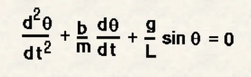
In the above equation,

g = gravity in m/s2,

L = length of the pendulum in m,

m = mass of the ball in kg,

b=damping coefficient.

Given initial condition:

L=1 metre,

m=1 kg,

b=0.05.

g=9.81 m/s^2

OBJECTIVES:

1. Solve ODE which represents equation motion of simple pendulum with damping with help of MATLAB code.
2. Understanding of ode45 in MATLAB
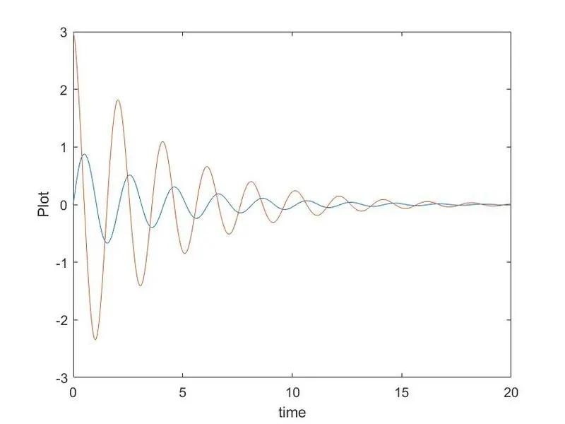
3. Plotting the graph of variation of angular displacements vs time , variation of angular velocity vs time.
4. Creating the animation plot of for motion of pendulum between motion between 0-20 sec, for angular displacement=0,angular velocity=3 rad/sec at time t=0.

θ=θ1">θ=θ1θ=θ1 ---(equation 1)

From equation 1:

dθdt=dθ1dt=θ2(equation2)">dθ/dt=dθ_1/dt=θ2 ---(equation2)

d2θ1dt2=ddt(dθ1dt)=dθ2dt(equation3)">(d^2)θ/d(t^2)=d/dt(dθ_1/dt)=d/dt(dθdt=dθ1dt=θ2(equation2)">θ2) ---(equation3)

From equation number 2,3:

dθ1dt=θ2(equation4)">dθ_1/dt=θ2 ---(equation4)

d2θ1dt2+bmdθ1dt+gLsin⁡θ=0">(d^2)θ/d(t^2) + (b/m)dθ/dt + (g/L)sinθ = 0

d2θ1dt2+bmdθ1dt+gLsin⁡θ=0">d2θ1dt2+bmdθ1dt+gLsin⁡θ=0">(d^2)θ_1/d(t^2) + (b/m)dθ_1/dt + (g/L)sinθ_1 = 0

d2θ1dt2+bmdθ1dt+gLsin⁡θ=0">d2θ1dt2+bmdθ1dt+gLsin⁡θ=0">(d^2)θ_1/d(t^2) = - (b/m)dθ_1/dt - (g/L)sinθ_1

dθ2dt=-bmθ2-gLsin⁡θ1(equation5)">d2θ1dt2+bmdθ1dt+gLsin⁡θ=0">d2θ1dt2+bmdθ1dt+gLsin⁡θ=0">dθ_2/dt = (−b/m) θ_2 − (g/L) sinθ_1 ---(equation5)

From equation 4 and 5

ddt[θ1θ2]=[θ2-bmθ2-g2sin⁡θ1]">d / dt[θ_1 ; θ_2]=[θ_2 ; −(b/m)θ_2 − (g/L) sinθ_1]

function [dtheta_dt]= ode_func(t,theta,b,g,l,m)

theta1=theta(1);

theta2=theta(2);

dtheta1_dt = theta2;

dtheta2_dt = -(b/m)*theta2-(g/l)*sin(theta1);

dtheta_dt=[dtheta1_dt;dtheta2_dt];

end

Main code:

clear all
close all
clc

b=0.05;
g=9.81;
l=1;
m=0.1;

% initial condition
theta_0=[0;3];
% time points
t_span=linspace(0,20,100);

% solve ODE
[t,results]=ode45(@(t,theta)ode_func(t,theta,b,g,l,m),t_span,theta_0);
plot(t,results(:,1))
hold on
plot(t,results(:,2))
xlabel('time');
ylabel('Plot');
% creating animation
ct=1;
theta_1=results(:,1);
for i=1:length(theta_1)

x0=0;
y0=0;
theta_2=theta_1(i);
x1=l*sin(theta_2);
y1=-1*cos(theta_2);
figure(2);
plot([-1 1],[0 0],'LineWidth',10,'color','g');
axis([-2 2 -2 2]);
hold on
line([x0 x1],[y0 y1],'linewidth',5,'color','b');
plot(x1,y1,'o','markersize',25,'MarkerFaceColor','r');
hold off
M(ct)=getframe(gcf);
ct=ct+1;
end
%creating movies
movie(M)
videofile=VideoWriter('ode_main.avi','Uncompressed AVI');
open(videofile);
writeVideo(videofile,M)
close(videofile);

Explanation:

• I have used clear all, close all and clc to clear all the varaibles, values and the plot that has been created in the previous code.
• I have assumed the gravity g=9.81 m/s^2, length of the pendulum L=1 m, mass of the ball m=1 kg, damping coefficient, b=0.05.
• I have used the plot command plot the coordinates.
• I have given axis for the given cordinates and end up with end.
• I have used the pause command to play the video in a time interval of 0 to 20.
• I have used the getframe command to capture each frame,videofile helps to name the file and formate of video.
• The matlab can generate the movie with all the frame in 'M'.
• I have used the videofile command to save the video as 'ode_main'(title) and in the 'Uncompressed AVI'(format).
• I have open the videofile using open command.
• I have write the videofile using write command.
• I have closed the videofile using close command.

Graph:

From above graph it can be observed that oscillation of pendulum are gradually damped as we can observe that angulalar displacement and angular velocity was gradually decreasing with time.

Google drive link:

https://youtu.be/u3naS1jK2lw