Week 4.1 - Solving second order ODEs

The main code :-

clear all
close all
clc

%inputs
b=0.05; 
g=9.81;
l=1;
m=0.1;

%initial condition
theta_0 =[0;3];

%time points
t_span = linspace(0,20,300);

%solve ODE
[t, results] = ode45(@(t,theta)ode_func(t,theta,b,g,l,m),t_span,theta_0);

% plotting
figure(1)
% plotting the 'Time vs Angular displacement'
subplot(2,1,1);
plot(t,results(:,1),'color','r','linewidth',1.5)
xlabel('Time [sec]');
ylabel('Angular Displacement [Rad]');
legend('Time vs Angular Displacement');
title('second order ODE');
grid on
subplot(2,1,2);
plot(t,results(:,2),'color','g','linewidth',1.5)
xlabel('Time [sec]');
ylabel('Angular Velocity [Rad/sec]');
legend('Time vs Angular Velocity');
grid on

%animation of the simple pendulum, placing the 'fixed point at (0,0)

X0=0;
Y0=0;
figure(2) % showing another window of image
videofile=VideoWriter('simple_pendulum','Uncompressed AVI'); %create video file using 'videowriter' command
open(videofile) %open video file

ct=1; %counter variable actually represent each and every frame
%using for loop for the 'repeating opration'
for i=1:length(t_span)
    %using the trignomertic equation find out (X1,Y1)
    X1=l*sin(results(i,1));
    Y1=-l*cos(results(i,1));
    %plotting the 'support rod' between (-0.5,0.5)
    plot([-0.5 0.5],[Y0 Y0],'linewidth',3);
    hold on;
    plot(X1,Y1,'marker','o','markersize',25,'markerfacecolor','r');
    plot([X0 X1],[Y0 Y1],'linewidth',1);
    axis([-2 2 -2 2]) %lable the x-axis(-2 2) y-axis(-2,2)
    grid on;
    title('damping of simple pendulum using second order ODE') %title of the graph
    legend('support rod','ball of pendulum','length of pendulum');%legend 'naming of the graph names'
    pause(0.05) %time pause
    M(i)=getframe(gcf); %get current figure
    ct=ct+1; %counter variable adding the next counter variable to creat video
    writeVideo(videofile,M(i)); %capture the figure in video file
    clf; % clear figure
end
movie(M) %movie file
close(videofile); %close the video file
    
    

Function code "ode_func" :-

function [dtheta_dt] = ode_func(t,theta,b,g,l,m)

theta1=theta(1);
theta2=theta(2);
dtheta1_dt=theta2;
dtheta2_dt=-(b/m)*theta2-(g/1)*sin(theta1);
dtheta_dt=[dtheta1_dt;dtheta2_dt];
end

Output :-

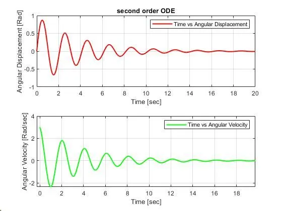
1) Plot :-

2) Animation video:-

https://youtu.be/m6XwgoDeT3c

Code Explanation :-

In the start of the code I give all the necessary inputs of g = gravity in m/s2, L = length of the pendulum in m, m = mass of the ball in kg, b=damping coefficient, t = time span in sec, theta = angular velocity in rad/sec as given in the question.

Made a function file named "ode_func" where the second-order ODE is converted in the form of two first-order equations.

Then I used an ode45 which is an inbuilt function of Matlab to solve the ODE and gave all the inputs to it.

Now for plotting, i made figure 1 and use the subplot command so that i can plot two different plots in single plot.

So in the first sub plot I plot figure for Time vs Angular Displacement and in second sub plot i plot the Time vs Angular Velocity plot.

And then for animation, i created another figure window Then using VideoWriter command i made an uncompressed AVI file named 'Simple_pendulum'.

Then i open the file made a counter variable ct and with help of for loop i calculated the position of X1 and Y1 for every point. Then i plotted and saved every plot in M metrix then using M metrix and WriteVideo function i made the animation video file. Then end the loop and close the video file.

Errors faced while programming :-

1)

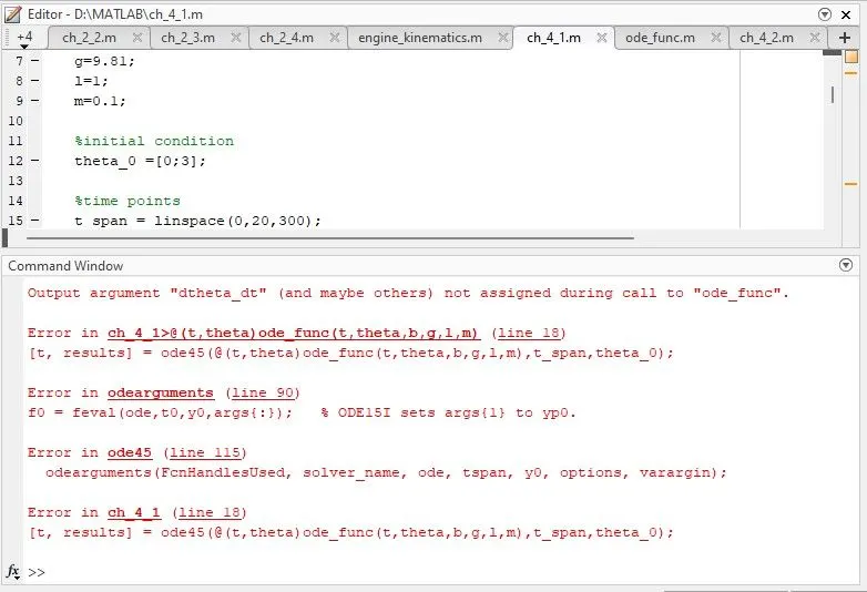
I got so many small errors and problems while Writing the code from which one of the error screenshot is attached. In this error, i tried to solve the error by reading the error massage and going to the error line mention in the error. It was so small error as i misspelled/typing error in one of the variable name in function file but it took mutch time and effort of me as its mot directly mentioned in error massage.

and Then i got difficulties in the animation part but the mentor in one on one session help me with that and i also refer robotic arm challenge code for Writing the animation part of the code.