Project 2 - Rankine cycle Simulator
Code to create a Rankine Cycle Simulator:-
In this code, we are using the standard Xsteam library to get the steam table data for water which is to be used to calculate the points in between the state variables.
To calculate the Rankine cycle data we have to input the given data in a command window.
Turbine Inlet temperature, t1 = 400° C
Turbine Inlet Pressure, p1 = 30 bars
Turbine Outlet Pressure, p2 = 0.05 bars = Condenser Inlet Pressure, p3
Main code :-
clear all
close all
clc

% displaying rankine cycle simulator and its processess

disp("__________Rankine cycle simulator__________")
fprintf('\n 1-2  is the  isentropic expansion process')
fprintf('\n 2-3  is the constant pressure heat rejection process')
fprintf('\n 3-4  is the isentropic compression process')
fprintf('\n 4-1  is the constant pressure heat addition process')

% variables for stage1

p1 = input ('Enter the Pressure at the Turbine Inlet (in bar): ')
t1 = input('Enter the Temperature at the Turbine inlet (in Degree celsius): ')
h1 = XSteam('h_pT',p1,t1);
s1 = XSteam('s_ph',p1,h1);
fprintf('\n\n _________Results________')
fprintf('\n\n At state point 1')
fprintf('\n P1 is:%f bar',p1)
fprintf('\n T1 is:%f deg celcius',t1)
fprintf('\n H1 is:%f KJ/Kg',h1)
fprintf('\n S1 is:%f KJ/KgK',s1)


% variables for stage2

p2 = input('Enter the Pressure at the Condenser (in bar): ')
s2 = s1;
p3 = p2;
t2 = XSteam('T_ps',p3,s1);
sf2 = XSteam('sL_p',p2);
sg2 = XSteam('sV_p',p2);
hf2 = XSteam('hL_p',p2);
hg2 = XSteam('hV_p',p2);
x = ((s2 - sf2)/(sg2 - sf2));
h2 = hf2 + (x*(hg2 - hf2));
v2 = XSteam('v_ph',p2,h2);
fprintf('\n\n At state point 2')
fprintf('\n P2 is:%f bar',p2)
fprintf('\n T2 is:%f deg celcius',t2)
fprintf('\n H2 is:%f KJ/Kg',h2)
fprintf('\n S2 is:%f KJ/KgK',s2)

% variables for stage3

t3 = t2;
p3 = p2;
s3 = XSteam('sL_p',p3);
h3 = XSteam('hL_T',t3);
v3 = XSteam('v_ph',p3,h3);
fprintf('\n\n At state point 3')
fprintf('\n P3 is:%f bar',p3)
fprintf('\n T3 is:%f deg celcius',t3)
fprintf('\n H3 is:%f KJ/Kg',h3)
fprintf('\n S3 is:%f KJ/KgK',s3)

% variables for stage4

s4 = s3;
v4 = v3;
p4 = p1;
h4 = XSteam('h_ps',p4,s4);
t4 = XSteam('T_hs',h4,s4);
fprintf('\n\n At state point 4')
fprintf('\n P4 is:%f bar',p4)
fprintf('\n T4 is:%f deg celcius',t4)
fprintf('\n H4 is:%f KJ/Kg',h4)
fprintf('\n S4 is:%f KJ/KgK',s4)


% variables for stage5

p5 = p4;
t5 = XSteam('Tsat_p',p5);
h5 = XSteam('hL_T',t5);
s5 = XSteam('sL_p',p5);
fprintf('\n\n At state point 5')
fprintf('\n P5 is:%f bar',p5)
fprintf('\n T5 is:%f deg celcius',t5)
fprintf('\n H5 is:%f KJ/Kg',h5)
fprintf('\n S5 is:%f KJ/KgK',s5)


% variables for stage6

t6 = t5;
p6 = XSteam('psat_T',t5);
s6 = XSteam('sV_T',t6);
h6 = XSteam('hV_T',t6);
fprintf('\n\n At state point 6')
fprintf('\n P6 is:%f bar',p6)
fprintf('\n T6 is:%f deg celcius',t6)
fprintf('\n H6 is:%f KJ/Kg',h6)
fprintf('\n S6 is:%f KJ/KgK',s6)

% loop to find variables on saturation lines

t = linspace(0,400,1000);
for i=1:length(t)
s_line1(i)=XSteam('sL_T',t(i));
end

for j=1:length(t)
s_line2(j)=XSteam('sV_T',t(j));
end
for i=1:length(t)
h_line1(i)=XSteam('hL_T',t(i));
end

for j=1:length(t)
h_line2(j)=XSteam('hV_T',t(j));
end

% net work output calculation

w_turbine = h1 - h2;                          % work done by turbine
w_pump = h4 - h3;                             % work taken by pump
work = w_turbine - w_pump;                    % net work output
q_in = h1 - h4;                               % heat addition
q_out = h2 -h3;                               % heat rejection

% thermal efficiency
n = work/q_in;

%Back work ratio
BWR = w_pump/w_turbine;

% Specific steam consumption
ssc = 3600/work;

%plotting T-S graph
figure(1)
hold on
plot([s_line1 s_line2],[t t],'linewidth',2)
plot([s1 s2 s3 s4 s5 s6 s1],[t1 t2 t3 t4 t5 t6 t1],'linewidth',2)
text(s1,t1,'1')
text(s2,t2,'2')
text(s3,t3,'3')
text(s4,t4,'4')
text(s5,t5,'5')
text(s6,t6,'6')
title("Rankine cycle T-S Diagram")
xlabel('Entropy(KJ/KgK)')
ylabel('Temperature(K)')
axis([0,8,0,450])

%plotting H-S graph
figure(2)
hold on
plot([s_line1 s_line2],[h_line1 h_line2],'linewidth',2)
plot([s1 s2 s3 s4 s5 s6 s1],[h1 h2 h3 h4 h5 h6 h1],'linewidth',2)
text(s1,h1,'1')
text(s2,h2,'2')
text(s3,h3,'3')
text(s4,h4,'4')
text(s5,h5,'5')
text(s6,h6,'6')
title("Rankine cycle H-S Diagram")
xlabel('Entropy(KJ/KgK)')
ylabel('Enthalpy(KJ/Kg)')
axis([0,8,0,3500])
Explaination :-
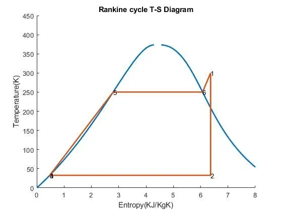
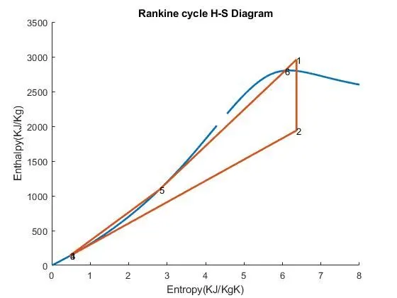
We displayed – the Rankine cycle simulator, using disp command, and then write the ranRankinele’s all process using fprintf command. Take input from user of Required parameters using input command, for example, Turbine inlet pressure(p_1) = 30 bar, Turbine inlet temperature(t_1) = 400 deg celsius ,Turbine outlet pressure(p_2) = 0.05 bar. Take required data from standard XSteam.m file which is in the same directory by calling the XSteam function with suitable arguments to find the values of enthalpy, entropy for state 1. Used fprintf command to print values of variables we found. Repeat the procedure for all other states until the last stage which is the sixth stage to find unknow parameters. Now we apply a for loop to find values of enthalpy and entropy at saturated temperature and store them into 's_line1', 's_line2", 'h_line1' and 'h_line2' variables. Find net work output and back work ratio with suitable formulas. Plot the T-s and h-s diagram using all the value we have found in different states and give proper x and y label and add state number by text command. Plot saturation line using the values we have found by for loop.
Output in command window :-
__________Rankine cycle simulator__________
1-2 is the isentropic expansion process
2-3 is the constant pressure heat rejection process
3-4 is the isentropic compression process
4-1 is the constant pressure heat addition processEnter the Pressure at the Turbine Inlet (in bar): 40
p1 =
40
Enter the Temperature at the Turbine inlet (in Degree celsius): 300
t1 =
300
_________Results________
At state point 1
P1 is:40.000000 bar
T1 is:300.000000 deg celcius
H1 is:2961.651480 KJ/Kg
S1 is:6.363849 KJ/KgKEnter the Pressure at the Condenser (in bar): 0.05
p2 =
0.0500
At state point 2
P2 is:0.050000 bar
T2 is:32.875490 deg celcius
H2 is:1939.514779 KJ/Kg
S2 is:6.363849 KJ/KgK
At state point 3
P3 is:0.050000 bar
T3 is:32.875490 deg celcius
H3 is:137.765119 KJ/Kg
S3 is:0.476254 KJ/KgK
At state point 4
P4 is:40.000000 bar
T4 is:32.985918 deg celcius
H4 is:141.766071 KJ/Kg
S4 is:0.476254 KJ/KgK
At state point 5
P5 is:40.000000 bar
T5 is:250.357519 deg celcius
H5 is:1087.426024 KJ/Kg
S5 is:2.796653 KJ/KgK
At state point 6
P6 is:40.000000 bar
T6 is:250.357519 deg celcius
H6 is:2800.897322 KJ/Kg
S6 is:6.069709 KJ/KgK>>
Output plots :-
1) T-S Diagram for Rankine cycle :-
2) H-S Diagram for Rankine cycle :-
Errors i got While coading :-
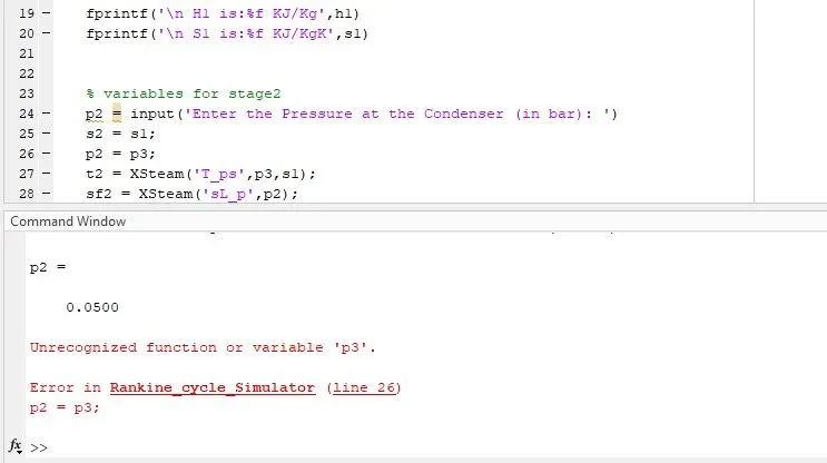
I have got so many Errors while Writing this code but it was the process of code because i was researching and making the code with trial and error method. Here i am attaching the screenshot of one of the small error i got in the code in this error it says that unrecognized function or variable 'p3'. I go to the error line and I have seen that i wrote it wrong and it should be p3=p2 and not p2=p3 then i corrected the code then run the code, like this I solved all the errors by solving them one by one.