Week 4.1 - Solving second order ODEs

AIM : 

To  write a program that solves the second order ODE

GOVERNING EQUATIONS : 

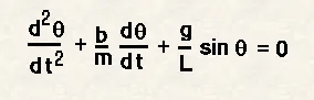
where 

g = gravity in m/s2

L = Length of the pendulum in meters

m = mass of the ball in kg

b=damping coefficient

OBJECTIVE : 

 To write a program that solves the following ODE. This ODE represents the equation of motion of a simple pendulum with damping

To Create an image that represents the position of the pendulum for each value of time

BODY OF THE CONTENT : 

1)PROGRAMMING LANGUAGE USED :

HTML( default )

2) CODE :

clear all
close all
clc
% Inputs
l=1 ;  % in metres

m=1; % in Kg

b=0.05 ; % damping coefficient 

g=9.81 ;  % in m/s^2

% Initial Conditions
theta_0 = [0 ;3];
% time points
t_span=linspace(0,20,500);
% solving ODE
[t,results] = ode45(@(t,theta)ode_func(t,theta,b,g,l,m),t_span,theta_0);

%Plotting

plot(t,results(:,1))
hold on
plot(t,results(:,2))

ylabel('Plot')
xlabel('Time(seconds)') 
title('Damped Harmonic Motion of a Pendulum')
legend('Angular displacement ', 'Angular velocity')


ct =1;
 for i = 1:length(results(:,1))
      x_start = 0  ;   
       y_start = 0 ;
        x_end = l*sin(results(i,1)) ;
         y_end = -l*cos(results(i,1)) ;

          % plotting the animation
           figure(2)
            plot([-1 1], [0 0], 'linewidth', 5)
             hold on
              plot([x_start x_end],[y_start y_end],'linewidth',3)
               hold on

                plot(x_end,y_end,'O','markersize',10,'markerFacecolor','g')
                 title('Animation of transient behaviour of a Pendulum')
                  axis([-3 3 -3 1])
                   pause(0.05)
                    hold off 

                     M(ct) = getframe(gcf)
                      ct = ct+1

 end


 % Animation of the pendulum
  movie(M)
  videofile=VideoWriter('Pendulum Animation.avi', 'uncompressed avi')
  open(videofile)
  writeVideo(videofile,M)
  close(videofile)

 SUPPLEMENTARY PROGRAM LIKE FUNCTION USED IN PROGRAMMING :

function [dtheta_dt] = ode_func(t,theta,b,g,l,m)

theta1= theta(1)
theta2= theta(2)
dtheta1_dt = theta2
dtheta2_dt = -(b/m)*theta2 - (g/l)*sin(theta1)
dtheta_dt = [dtheta1_dt; dtheta2_dt]
end 

 STEPWISE EXPLANATION OF CODE :

clear all

close all

clc

% Inputs

% defining the inputs as below

l=1 ;  % in metres          % length of the string = 1 meter

m=1; % in Kg.                 % mass of the ball=1 Kg

b=0.05 ; % damping coefficient .      % damping coefficients of damper system

g=9.81 ;  % in m/s^2.               % acceleration due to gravity 

% Initial Conditions

theta_0 = [0 ;3];.            %solution vector consists of values of initial displacement (here it is 0) and initial velocity (here it is 3)

% time points

t_span=linspace(0,20,500);.  %  creating time array from 0 to 200 with 500 values using linspace command

% solving ODE

[t,results] = ode45(@(t,theta)ode_func(t,theta,b,g,l,m),t_span,theta_0);

%ode45 is inbuilt command that solves  ordinary partial differential equations in matlab

@(t,theta).        %  main inputs where t and theta are dependent and independent variables of ODE system

%Plotting

plot(t,results(:,1))        % plots t vs displacement that is stored in results of 1st column

hold on        

plot(t,results(:,2))         % plots t vs velocity that stored in results of  2nd column

ylabel('Plot')        % labels  y axis as plot

xlabel('Time(seconds)') .    % time in second is taken as x axis

title('Damped Harmonic Motion of a Pendulum')

 % keeps the title of the plot 

legend('Angular displacement ', 'Angular velocity')

 % command that used to distinguish between angular displacement and angular velocity

ct =1;

 for i = 1:length(results(:,1)).         % used for loop 

to iterate the loop For each value in time

      x_start = 0  ;   defining starting x coordinate

       y_start = 0 ; defining the starting y cordinate

        x_end = l*sin(results(i,1)) ; % ending x cordinate

         y_end = -l*cos(results(i,1)) ;  % ending y cordinate

          % plotting the animation

           figure(2)

            plot([-1 1], [0 0], 'linewidth', 5)

             hold on

              plot([x_start x_end],[y_start y_end],'linewidth',3)

 % plotting using starting and ending cordinates providing first X coordinates and then the Y coordinates  of two points 

  hold on  % command that makes plots do not get over return

 % to close video file we used close command

       FUNCTION CODE EXPLAINATION :

        function [dtheta_dt] = ode_func(t,theta,b,g,l,m)

% ode function is the name of the function and the format used is for function definition

t, theta ,b ,g , l, m are the input parameters that are passing

theta1= theta(1)   %defining theta (1) as theta1 

theta2= theta(2) % defining theta(2) as theta2 to make the second order differential equation into single order differential equation

dtheta1_dt = theta2  % differentiating theta 1 with respect to time gives theta 2

dtheta2_dt = -(b/m)*theta2 - (g/l)*sin(theta1)

% after transforming second order differential equation into single order differential equation then dtheta2_dt becomes  { -(b/m)*theta2 - (g/l)*sin(theta1)}

dtheta_dt = [dtheta1_dt; dtheta2_dt]

% solution vector for theta is transformed into above when single order differential equation is written in matrix form

end 

 % end is a keyword that terminate function

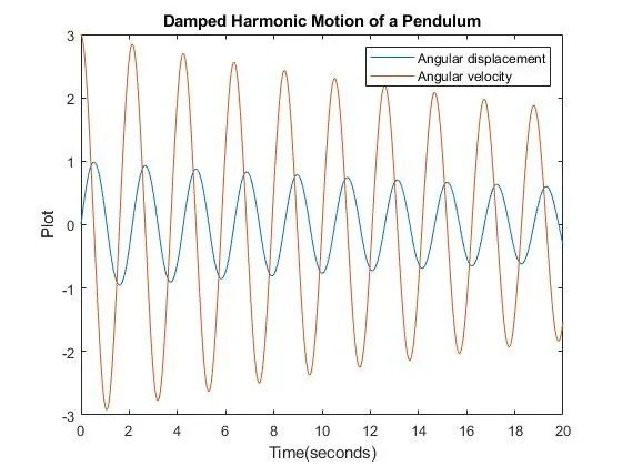
PLOTS :

 ANIMATION LINK  :

https://youtu.be/PumPK8NTm6I

CONCLUSION :

Hence , solved the second order differential equation that represents the equation of motion of simple pendulum under damping .