Challenge

Week 4.1 - Solving second order ODEs

NNikhil Kumar26 Jul 2023

Week 4.1 - Solving second order ODEs

PROBLEM STATEMENT

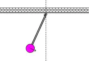
In Engineering, ODE is used to describe the transient behavior of a system. A simple example is a pendulum

The way the pendulum moves depends on the Newtons second law. When this law is written down, we get a second order Ordinary Differential Equation that describes the position of the "ball" w.r.t time.

Similarly, there are hundreds of ODEs that describe key phenomena and if you have the ability to solve these equations then you will be able to simulate any of theses systems.

Your objective is to write a program that solves the following ODE. This ODE represents the equation of motion of a simple pendulum with damping

In the above equation,

g = gravity in m/s2,

L = length of the pendulum in m,

m = mass of the ball in kg,

b=damping coefficient.

Write a program in Matlab\Octave that will simulate the pendulum motion, just like the one shown in the start of this challenge.

use,

L=1 metre,

m=1 kg,

b=0.05.

g=9.81 m/s2.

Simulate the motion between 0-20 sec, for angular displacement=0,angular velocity=3 rad/sec at time t=0.

When you do this you will get the position of the pendulum as a function of time. Use this information to animate the motion of the pendulum, as shown in the below figure.

SOLUTION WITH REPORT:-

The second order differential equation of a simple pendulum is :-

d^2theta/dt^2 + (b/m)dtheta/dt + g/L sin theta = 0 ....................(A)

Its a second order differential equation so we have to convert it into first order differential equation.

Lets say

theta = theta 1

d_theta = d_theta1/dt = theta_2 ....................(1)

d^2theta/dt^2 = d^2theta1/dt^2 = d/dt(dtheta1/dt) = d/dt(theta 2) ...................(2)

Substituting the eqn (2) to eqn (A).

dtheta 2 /dt + (b/m)theta 2 + g/L sin theta 1 = 0

d theta 1 / dt = theta 2

d theta 2/dt = - (b/m)theta 2 - g/Lsin theta 1.

so,

we got

theta 1(dot) = theta 2

theta 2(dot) = -(b/m)theta 2 - g/L sin theta 1

MATLAB PROGRAM

#maincode

clear all
close all
clc

%Inputs
b = 0.05; %damping coefficient
g = 9.81; %gravity in m/s^2
l = 1;    %length of the pendulum in m
m = 1;    %mass of thge ball in kg

%Initial conditions
theta_0 = [0,3];
%time plots
t_span = linspace(0,20,500);

%solve for ode
[t,results] = ode45(@(t,theta)my_func(t,theta,l,m,g,b),t_span,theta_0)



v = VideoWriter('pendulum.avi');
open(v);




for i=1:length(results(:,1))
    
    x1=l*sin(results(i,1));
    y1=-l*cos(results(i,1));
    
    plot([0,x1],[0,y1],'linewidth',3);
    hold on
    plot(x1,y1,'o','MarkerSize',15,'markerfacecolor','r');
    grid on
    axis([-1.5 1.5 -1.5 0.5]);
    pause(0.01);
    xlabel('plot')
    ylabel('time')
    title('Motion of Pendulum')
    frame = getframe(gcf);
    writeVideo(v,frame)
    hold off
    
end
close (v)

#functioncode

function [derivative] = my_func(t,theta,l,m,g,b)

derivative = zeros(2,1);
derivative(1,1) = theta(2);
derivative(2,1) = (-b/m)*theta(2)-(g/l)*sin(theta(1));



end

The above set of codes executes without an error.

OUTPUT :-

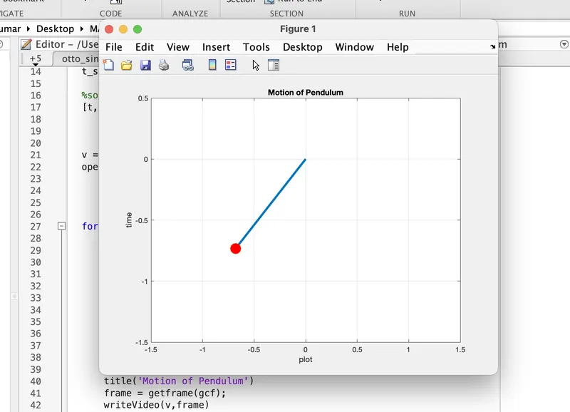
OUTPUT from the command Window

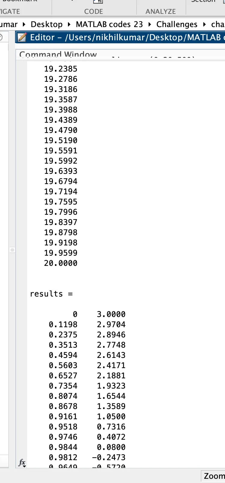
The above one is the values of the TIME array which has one column and the bottom one is the results which is containing the velocity array which has two columns.

VALUES IN THE WORKSPACE OUTPUTS

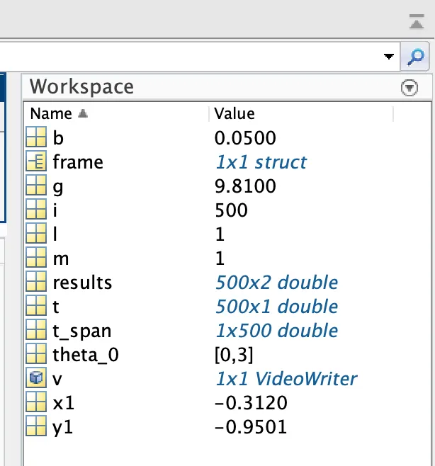
The required animation is being uploaded on the YOUTUBE and the link of the former is being provided here.

https://youtu.be/uMtWcX5Ldcc

STEP BY STEP EXPLANATION OF THE CODE

clear all, close all, clc: These are MATLAB commands used to clear the workspace, close all figures, and clear the command window.
%Inputs: These are comments indicating that the following variables are inputs to the system.
b = 0.05; %damping coefficient: The damping coefficient of the pendulum system.
g = 9.81; %gravity in m/s^2: The acceleration due to gravity in meters per second squared.
l = 1; %length of the pendulum in m: The length of the pendulum in meters.
m = 1; %mass of the ball in kg: The mass of the ball at the end of the pendulum in kilograms.
%Initial conditions: These are comments indicating that the following variable is the initial condition for the system.
theta_0 = [0,3];: An array representing the initial state of the system. Here, theta_0(1) is the initial angle (in radians) of the pendulum, and theta_0(2) is the initial angular velocity (in rad/s).
%time plots: This is a comment indicating the following variable represents the time span for which the simulation will be run.
t_span = linspace(0,20,500);: It creates an array of 500 time values from 0 to 20 seconds. This time span will be used for simulating the system.
%solve for ode: This is a comment indicating the following code segment solves the Ordinary Differential Equation (ODE) representing the pendulum's motion.
[t,results] = ode45(@(t,theta)my_func(t,theta,l,m,g,b),t_span,theta_0): This line uses the ode45 solver to numerically solve the ODE representing the pendulum's motion. It integrates the equations of motion over the given time span t_span, starting from the initial conditions theta_0, and returns time values t and the corresponding state variables (angle and angular velocity) in the results array.
v = VideoWriter('pendulum.avi');: It creates a video writer object named v to save the animation of the pendulum's motion.
open(v);: It opens the video writer for writing video frames.
for i=1:length(results(:,1)): This initiates a loop that iterates through the time steps of the simulation.
x1=l*sin(results(i,1));: It calculates the x-coordinate of the ball's position based on the pendulum angle at the current time step.
y1=-l*cos(results(i,1));: It calculates the y-coordinate of the ball's position based on the pendulum angle at the current time step.
plot([0,x1],[0,y1],'linewidth',3);: It plots a line representing the pendulum rod from the origin (0,0) to the current ball position (x1, y1).
hold on: This command makes sure that subsequent plots will be overlaid on the same figure.
plot(x1,y1,'o','MarkerSize',15,'markerfacecolor','r');: It plots a red circle representing the ball at its current position.
grid on: It displays the grid on the figure.
axis([-1.5 1.5 -1.5 0.5]);: It sets the limits of the plot to zoom in on the pendulum's motion within a specific range.
pause(0.01);: It adds a short pause between frames to slow down the animation.
xlabel('plot'): It sets the label for the x-axis of the plot.
ylabel('time'): It sets the label for the y-axis of the plot.
title('Motion of Pendulum'): It sets the title for the plot.
frame = getframe(gcf);: It captures the current figure frame for creating the video.
writeVideo(v,frame): It writes the captured frame to the video.
hold off: This command releases the hold on the plot, allowing the next iteration to plot the updated pendulum position.
end: The end of the loop.
close(v): It closes the video writer after all frames are written.
function [derivative] = my_func(t,theta,l,m,g,b): This defines a function my_func that calculates the derivatives of the state variables (angle and angular velocity) of the pendulum system.
derivative = zeros(2,1);: It initializes the derivative array to store the derivatives of the state variables.
derivative(1,1) = theta(2);: The first element of derivative represents the derivative of the angle, which is equal to the angular velocity (theta(2)).
derivative(2,1) = (-b/m)*theta(2)-(g/l)*sin(theta(1));: The second element of derivative represents the derivative of the angular velocity. It is calculated based on the damping term (-b/m * theta(2)) and the gravitational restoring force term (-(g/l)*sin(theta(1))).

That's the line-by-line explanation of the given MATLAB code, which simulates the motion of a pendulum and creates an animation of its movement.

Week 4.1 - Solving second order ODEs

Ship work like this
in your own course.

Talk to a career counsellor

Ship work like thisin your own course.

Talk to a career counsellor

Ship work like this
in your own course.