Week 4.1 - Solving second order ODEs

In Engineering, ODE is used to describe the transient behavior of a system. A simple example is a pendulum

The way the pendulum moves depends on the Newtons second law. When this law is written down, we get a second order Ordinary Differential Equation that describes the position of the "ball" w.r.t time.

Similarly, there are hundreds of ODEs that describe key phenomena and if you have the ability to solve these equations then you will be able to simulate any of theses systems.

Your objective is to write a program that solves the following ODE. This ODE represents the equation of motion of a simple pendulum with damping

In the above equation,

g = gravity in m/s2,

L = length of the pendulum in m,

m = mass of the ball in kg,

b=damping coefficient.

Write a program in Matlab\Octave that will simulate the pendulum motion, just like the one shown in the start of this challenge.

use,

L=1 metre,

m=1 kg,

b=0.05.

g=9.81 m/s2.

Simulate the motion between 0-20 sec, for angular displacement=0,angular velocity=3 rad/sec at time t=0.

When you do this you will get the position of the pendulum as a function of time. Use this information to animate the motion of the pendulum, as shown in the below figure.

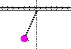
Your animation does not have to look exactly like this and here is the logic.

• For each value in time
• Create an image that represents the position of the pendulum
• You can assume the length of the string and the size of the ball
• Use the marker command to create a sphere
• One end of the pendulum is fixed
• The other end moves according to the solution of the ODE you had solved.
• If you are using using Matlab, use the movie command create an animation
• If you are using Octave you need to generate images first and then stitch them to form the animation

Aim: Solving a simple pendulum's second order ordinary differential equation and animating the damping effect.

Objective:

• To change an ordinary differential equation of second order into an equation of first order.
• Using the built-in MATLAB function for solving ordinary differential equations to create the function.
• To create a simple pendulum animation.

FACTORS ENTAILED:

• A simple pendulum is a mechanical arrangement that demonstrates periodic motion. The simple pendulum comprises a small bob of mass ‘m’ suspended by a thin string secured to a platform at its upper end of length L.

• The simple pendulum is a mechanical system that sways or moves in an oscillatory motion. This motion occurs in a vertical plane and is mainly driven by the gravitational force. Interestingly, the bob that is suspended at the end of a thread is very light somewhat we can say it is even massless. The period of a simple pendulum can be made extended by increasing the length string while taking the measurements from the point of suspension to the middle of the bob. However, it should be noted that if the mass of the bob is changed will the period remains unchanged. The period is influenced mainly by the position of the pendulum in relation to Earth as the strength of the gravitational field is not uniform everywhere.

• By applying Newton’s second law motion we can obtain the equation of motion for a simple pendulum which is given as:
• d2θdt+bmdθdt+gLsinθ=0">d2θdt+bmdθdt+gLsinθ=0

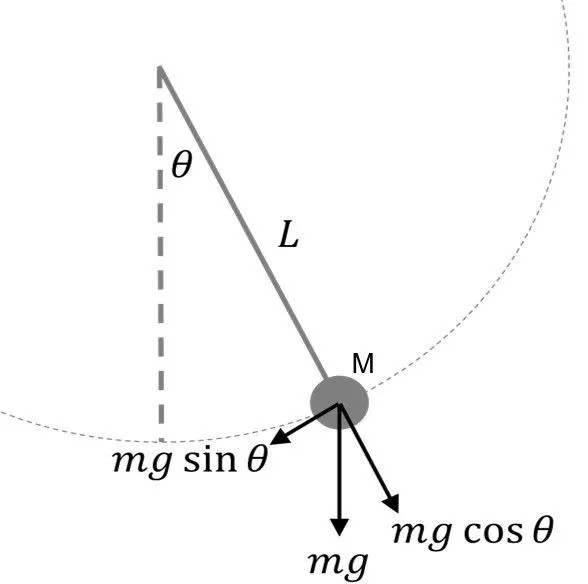
• The equation must be changed from a second-order partial differential equation to a first-order differential equation in order to be solved in MATLAB using the "ode45" function. we get,

θ′1=θ2">θ'1=θ2and θ′2=-(bmθ2)-gLsinθ1">θ'2

Code Explanation:

• The input data from the problems represent the code's initial inputs. The time domain for which the entire code will run is then created. The command "linspace" was used, with a range of 0 to 30 seconds and a value of 100 in between.

• Then, because we need to calculate both values from the equation of motion for plotting purposes, we give the initial conditions for the angular displacement and velocity in column vector form.

• The code includes a function that is used inside the main code to solve the second-order differential equation. Another function in the main code computes the array of time and displacement data.

• After calculation plotting is done in which subplot command is used, Then, after saving the movie, we created a for loop for which we are creating the frame motion for the straightforward pendulum.

Matlab Program:

%given data
%damping coefficient
b = 0.05; 
%acceleration due to gravity  
g = 9.81;
%length of Pendulum in meters   
l = 1;
%mass      
m = 1;       
%time duration for simulation 
t_s = linspace(0,30,100);
%angular displacement & velocity
y_starting = [0;3];

%using ODE45
a = @(t,y)ode_second_order_pendulum(y,b,m,l,g);
[t,y]= ode45(a,t_s,y_starting);

%Plot of angular displacement & velocity w.r.t time function.
figure(1);
grid on
subplot(1,2,1)
plot(t,y(:,1));
title('Displacement vs Time');
xlabel('Time in seconds');
ylabel('Angular displacement in rad');
subplot(1,2,2)
plot(t,y(:,2));
title('Angular velocity Vs Time')
xlabel('Time in seconds');
ylabel('Angular velocity in rad/sec');
grid off
saveas(figure(1),'subplot','jpg')

%polar co-ordinate to cartesian co-ordinate
y1 = -1*cos(y(:,1));
x1 = 1*sin(y(:,1));

%video for pendulum motion
for i = 1:100
    figure(2)
    plot([0 x1(i)],[0 y1(i)],'linewidth',3,'color','r');
    hold on
    plot(x1(i),y1(i),'marker','o','linewidth',10,'markerfacecolor','g');
    plot([-1.2 1.2],[0 0],'linewidth',3,'color','b');
    axis([-1.2 1.2 -1.2 1.2]);
    title(['Time: ', num2str(t_span(i))]);
    M(i) = getframe(gcf);
    close(2)
end

movie(M)
videofile = VideoWriter('simplependulum.avi','Uncompressed AVI');
open(videofile);
writeVideo(videofile,M)
close(videofile)

The Function is given as follows;

function ydot = ode_second_order_pendulum(y,b,m,l,g)

ydot = [y(2);-(b/m)*y(2)-(g/l)*sin(y(1))];

end

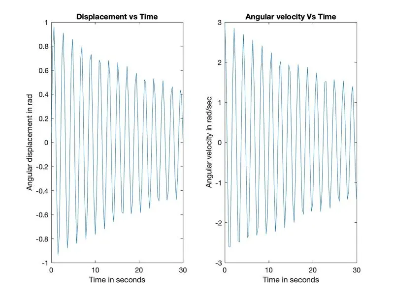
Output:

• The graph illustrates that the damping factor causes the displacement to reduce as we advance in time. The plot makes it clear that displacement starts at 0 as the initial condition. The angular velocity vs. time plot shows that it began at 3 rad/sec and has since dropped significantly.