Week 4.1 - Solving second order ODEs
Aim: To solve 2nd order ODE equation and share the animation youtube link of pendulum.
Objective:
Our objective is to write a program that solves the following ODE.
The following ODE represents the equation of motion of a simple pendulum with damping.
(d ^ 2 * theta)/(d * t ^ 2) + b/m * d/dt (theta) + g/L * sin theta = 0
where,
g = gravity in m/s2,
L = length of the pendulum in m,
m = mass of the ball in kg,
b = damping coefficient.
Given Data:
L = 1 meter,
m = 1 kg,
b = 0.05.
g = 9.81 m/s2.
At initial condition, time = 0, angular displacement = 0, angular velocity = 3 rad/s^2.
Time span = 0 to 20 seconds.
MATLAB/ Octave has standard solver for solving ordinary differential equations (ODEs) the function is "ODE45". This function calculate solutions of ODEs by using Numerical method.
(d ^ 2 * theta)/(d * t ^ 2) + b/m * d/dt (theta) + g/L * sin theta = 0
Output = ode45("Function", "time", "Initial condition")
For coding we are using ODE45 solver. In following code an anonymous function f(t,theta) is used.
here, consider angular displacement = theta = theta(1)
The ODE function :
The function is used for the differenciation of the given data
function [dtheta_dt]= ode_func
theta1 = theta(1)
theta2 = theta(2)
dtheta1_dt = theta2;
dtheta2_dt = -(b/m)*theta2 - (g/1)*sin(theta1);
dtheta_dt = [dtheta1_dt; dtheta2_dt];
end
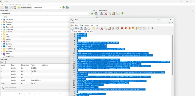
Program with explination
clear all
close all
clc
l=1; [%Length of pendulum string in meter]
m=1; [%Mass of pendulum in kg]
b=0.05;[ %Damping coefficient]
g=9.81; [%Gravitational acceleration in (N/m^2)]
t=linspace(0,20,100); [%time span 0 to 20 seconds with 100 time steps].
theta0=[0 3]; [%initial conditions [angular displacement Angular velocity]
[%Ordinary differential equation function]
[t, theta]= ode45(@(t,theta) [theta(2) ;
-(b*theta(2)/m)-(g*sin(theta(1))/l)], t, theta0);
[%Here theta is angular displacement which is shown by theta(1)
[%Rate of change of theta is angular velocity which is shown by theta(2)]
[%Rate of change of theta(2) is angular acceleration]
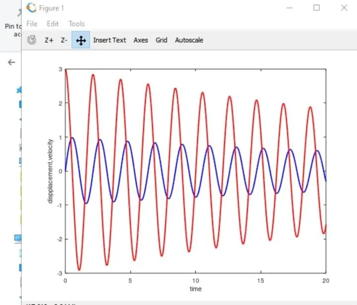
[% Creation of graph resulting magnitude of angular velocity & displacement w.r.t time]
figure(1);
plot(t,theta(:,1),'color','b'); %plotting time v/s angular displacement
hold on;
plot(t,theta(:,2),'color','r'); %plotting time v/s angular velocity
legend('Angular displacement','Angular velocity');
xlabel('Time (Seconds)');
ylabel('Magnitude');
title('Pendulum plot for angular displacement & angular velocity')
for i= 1:length(theta(:,1))
figure(2)
clf;
[%origin of pendulum (x0,y0)(Constrain point)]
x0=0;
y0=0;
[% Other end of pendulum (x1,y1) (Centre of bob)]
x1=l*sin(theta(i,1));
y1=l*cos(theta(i,1));
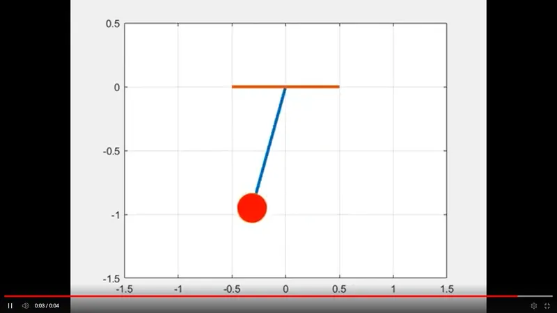
plot([-1 1], [0 0]);
hold on;
line([x0 x1], [-y0 -y1]);
plot(x1,-y1,"0",'markersize',40,'markerfacecolor','g'); % Plotting of bob
grid on;
axis([-1.5 1.5 -1.5 0.5]); %axis dimensions
title('Pendulum animation');
printf('Creating GIF- Progrss... %d/%dn', i, length(t));
img = print('-RGBImage');
imwrite(img, 'animation.gif', 'DelayTime', 0.1,'Compression','bzip','WriteMode','append');
endfor
Screenshot:
Youtube link:
https://youtu.be/7T5UQDiPab0