Week 4.1 - Solving second order ODEs

This video is about solving the second order differential equation using programming. Many mechanical systems can be modelled using the second order differential equation using programming. Examples are spring-mass system, damper-spring mass system and vehicle suspension system can be modelled using the second order differential equations. The equation is solved by breaking down a second order ODE into a series of first order ODEs. A second order is solved by breaking down into two first order ODEs and getting into matrix.

Transient Behaviour

The transient behaviour is observed in many natural phenomena and also many engineering systems can be modelled by solving the equations obtained through transient analysis.

The equations generally obtained are Ordinary Differential Equations where there is one or more dependent and also the independent variable, usually time.

• A simple example is that of a pendulum motion where the behaviour of the motion of the pendulum about an axis line is time varying.
• The pendulum motion can be analysed by applying Newton's Second Law to he motion of the bob.
• The string is like supplying the requied restoring force to get back the pendulum into the equalibrium position after it is given an initial displacement and velocity.

• ,

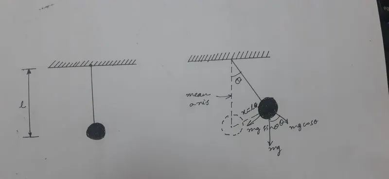
• When this law is applied to the bob of the pendulum,we get a Second order Differential Equation.

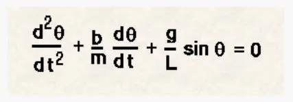
• The other examples of the motion are the spring mass system whrein the vehicle dynamics can be modelled using the spring mass system using a damper.
• There are many other systems and key phenomena that can be modelled using Ordinary Differential Equations and hence the techniques developed for the same can be used to get useful results of the behaviour of the systems.
• Techniques developed can be both analytical and computational.
• With the use of the software solvers the equations can be solved computationally very easily reducing effort to a great extent and also saving time.
• The fundamental idea in computationally solving lies in breaking down the high oreder ODE into a set of first order differential equations.

• After breaking down to a set of first order ODEs the dependent variables are arranged as a coloumn vector and the solution is obtained by integrating over the range of the independent variable.

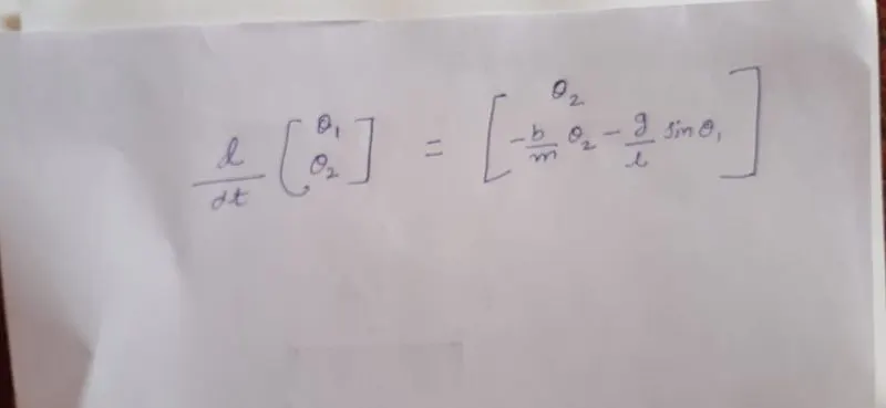
• A simple pendulum example is taken here to solve the equations computationally.
• Here the second order differential equation is broken down into two first oreder ODEs.
• A third order ODE can be broken down into three first order ODEs and can be integrated over time.
• ODE45 is used to solve the ODE of the simple pendulum.
• It is MATLAB's standard solver for ordinary differential equations(ODEs) is the function ode45.
• This function implements a Runge-Kutta method to computationally integrate over the independent variable.

Main Script:

1. Open MATLAB and click 'new script'

2. Add function in the name of 'dtheta_dt"

function[dtheta_dt] = odefunc(t,theta,b,g,l,m)

3. theta1 and theta2 are assigned as follows to avoid confusion:

theta1 = theta(1);

theta2 = theta(2);

4. the set of odes converted are written as follows:

dtheta1_dt = theta2;

dtheta2_dt = ((-b/m)*theta2)-((g/l)*sin(theta1));

5.both odes are written in the form of a column matrix.

dtheta_dt = [dtheta1_dt; dtheta2_dt];6. by combining them in a single array, we get the final equation for solving ode.

Execution Script:

1. Program is written to call the function and the graph and motion are plotted.

2. usual comments are added

clear all % clears all the variables

close all % closes all the plots and figures

clc % clears the command window

3. the parameters are added which are damping coefficient,gravity,length and mass of the bob

b = 0.05;

m = 0.1; % mass of the pendulum in kg

g = 9.81; % acceleration due to gravity

l = 1; % length of pendulum in metres

5. the values of time are given over which the ode is integrated and a set of time values are chosen to simulate the motion between ' 0 - 20s'. 'linspace' command is used for this.

t_span = linspace(0,20,500);

6. the problem is initialised with the initial values to the two dependent variables ,first one for 'angular displacement- theta1' and second one for 'angular velocity- theta2'

strt = [0 ; 3];

7. Having got all the inputs for solving the ode function, 'ode 45' statement is used to solve the equation

[time, derivatives] = ode45(@(t,theta) odefunc(t, theta, b,g,l,m),t_span,strt);

'ode45' is an inbuilt solver in MATLAB and @(t,theta) contains two main inputs of a differential equation. Later, the function 'odefunc' is defined with inputs that are needed for solving. Motion time and initial values are given respectively according to the syntax of the function ode45.

8. the angular displacement values are plotted against time,'plot' command is used as it can be continued to use for 'angular velocity vs time' curve.

figure(1)

plot(time,derivatives(:,1),'r')

9. 'hold on' is used so that the plots of 'angular displacement' vs time and 'angular velocity vs time' can be seen together.

hold on

10. the plot of angular velocity vs time is obtained.

plot(time, derivatives(:,2),'b')

11. 'xlabel' and 'ylabel' are used for labelling the axis. time is taken on the x axis and the dependent variables on y axis.

xlabel('time')

ylabel('derivatives')

12. 'title' command is used for naming the plots.

title('Plots of displacement and velocity wrt time')

13. legend command is used to name and differentiate the plots

legend('disp-time', 'velocity-time')

14. The motion of a simple pendulum is to be plotted now. counter variable is defined for the for loop to transfer the frames of the motion which we get while running the code to an array and create the video of the simple pendulum.

ct = 1;

for i = 1: length(derivatives(:,1))

15. The origin about the which the pendulum is pivoted is fixed with 'x0' & 'y0'

xo = 1.5;

yo = 2;

16. The coordinates of the end of the centre of mass of the bob at different locations of the motion are taken by this and used in the 'plot' command. the sine angle should be properly taken. *ERROR

x1 = 1.5-l*sin(derivatives(i,1));

y1 = 2 - l*cos(derivatives(i,1));

17. This figure window is used to capture the motion of the bob in different time frames.plot command is used to join at different time frames.plot a line which represents the thread in black colour.

figure(2)

plot([xo x1],[yo y1],'color','black')

18. hold on prevents the previous plot to get rewrited.

hold on

19. draw a line to represent the ceiling or the base/support at the top

plot(x1,y1,'o','Markersize',20,'color','b','MarkerFaceColor','r','MarkerEdgeColor','magenta')

21.hold off is used to stop the figure.

hold off

22. the axis of the plots plotted is given

axis([-1.5 4 -3 3])

23. pause command is given to have a time gap between each frame of the plots

pause(0.01)

24. All the frames are inserted to combine the figures and an array 'M' is created.

M(ct) = getframe(gcf);

25. the counter variable is incremented to get fresh plots at each time frame.

ct = ct+1;

26. finally, we exit the 'for' loop.

end

% creating animation

27. The array 'M' earlier obtained which contained all the time frames is converted to a motion i.e into a video which is in AVI.

movie(M)

Videofile = VideoWriter(final_pendulum_motion.avi,"Uncompressed AVI")

Open(Videofile)

writeVideo(Videofile,M)

close(Videofile)

clear all
close all
clc

b = 0.05;
m = 1;
g = 9.81;
l = 1;
t_span = linspace(0,10,500);
strt = [0; 3];

[time,derivatives] = ode45(@(t,theta) odefunc(t,theta,b,g,l,m),t_span, strt);
figure(1)
plot(time, derivatives(:,1),'r')
hold on
plot(time, derivatives(:,2),'b')
xlabel('time')
ylabel('derivatives')
title('Plots of displacement and velocity wrt time')
legend('disp-time','velocity-time')
hold off

ct = 1
for i = 1:length(derivatives(:,1))
    x0 = 1.5;
    y0 = 2;
    x1 = 1.5- l*sin(derivatives(i,1));
    y1 = 2- l*cos(derivatives(i,1));
    figure(2)
    plot([x0 x1],[y0 y1], 'Color','black')
    hold on
    plot(x1,y1,'o','Markersize',20,'color','b','MarkerFaceColor','r','MarkerEdgeColor','magenta')
    axis([-1.5 4 -3 3 ])
    pause(0.01)
    M(ct) = getframe(gcf);
    ct = ct+1
    hold off
end
    %creating animation
    Movie(M)
    Videofile = VideoWriter('final_pendulum_motion.avi',"Uncompressed AVI")
    Open(Videofile)
    writeVideo(Videofile,M)
    close(Videofile)

function[dtheta_dt] = odefunc(t,theta,b,g,l,m)
theta1 = theta(1);
theta2 = theta(2);
dtheta1_dt = theta2;
dtheta2_dt = (-b/m)*theta2-(g/l)*sin(theta1);
dtheta_dt = [dtheta1_dt;dtheta2_dt];
end

Output in the command window:

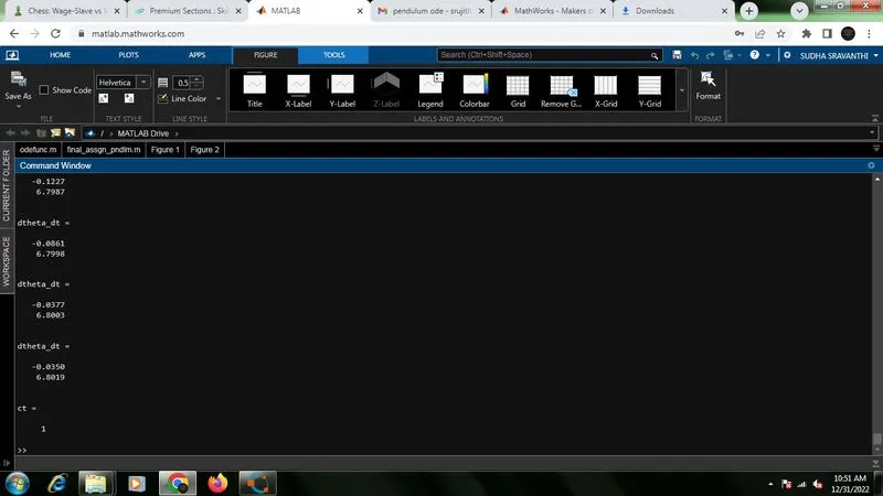
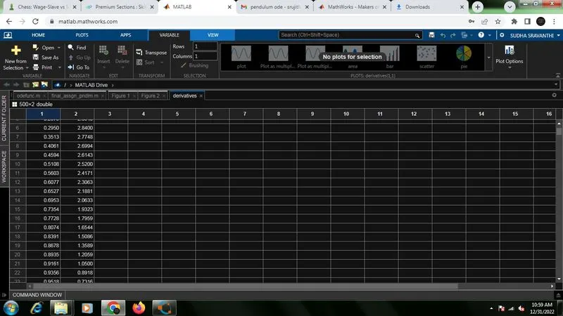
results:First column represents the angular displacement and the second column represents the angular velocity. We get 500x2 matrix.

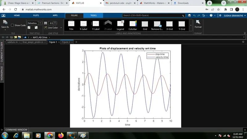
Output plots of codes: Two curves are represented in the time interval of 0-20 seconds. Red line represents angular displacement- time curve and blue line represents velocity-time curve.

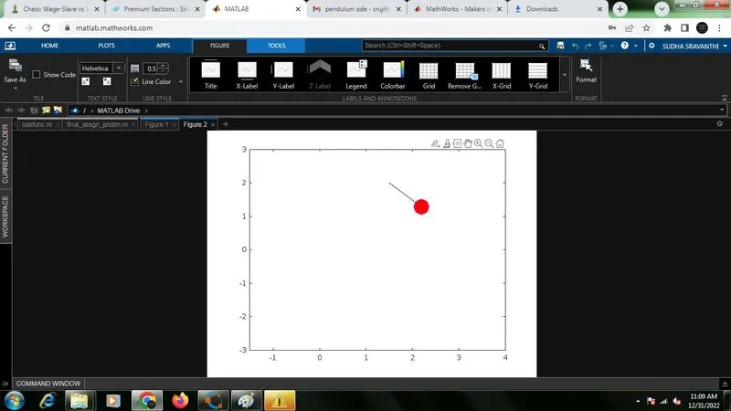
the output of figure(2) : the output when the whole program is run.

Errors faced while programming:

use of sind(derivatives) and cosd(derivatives) instead of sin(derivatives) and cos(derivatives)

we could not get clear motion of the pendulum as with the given parameters the solution (angular displacement and angular velocity) is to be taken in radians and not be converted to degrees.

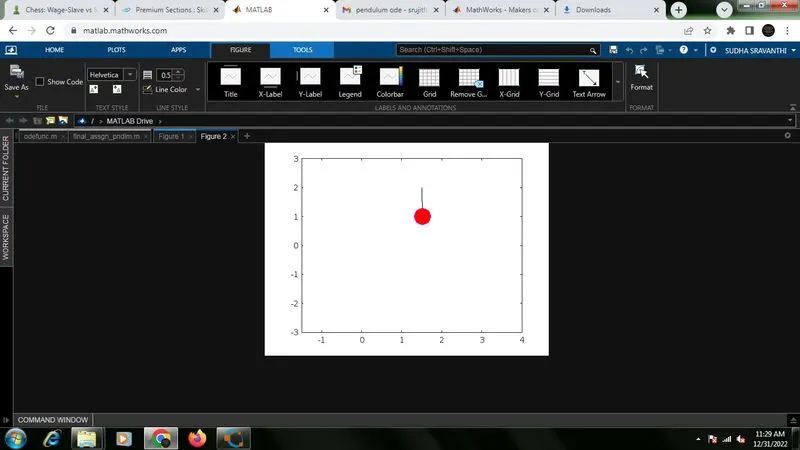
error rectification: the error is rectified by taking the sin(derivatives(:,1)) and cos(derivatives(:,1) instead of sind(derivatives(:,1) and cosd(derivatives(:,1))

The video link is given below:

https://youtu.be/kA6FG_WsyV8

Points to remember:

1. The function file name(.m file) should be taken same as the function called in the solver ode 45.

2. The set of values given for b,g,l,m (0.05,9.81,1,1) resp. are consistent to execute a simple harmonic motion according to the second order differential equation.

3. The sine and cosine is to be taken with the angle value in radians and not converted to degrees.