Project 2 - Rankine cycle Simulator

Rankine Cycle and the Thermodynamics:

Rankine cycle is a power cycle where steam is the working fluid. It is one of the most important power cycle as it is widely used to generate large amount of power (mechanical work output). Following the similar guidelines as the Carnot cycle, a Rankine cycle also has four main thermodynamic processes out of which two may be observed as which ‘Work’ is involved as the Energy transit while the other two are the thermodynamic processes where ‘Heat’ is the energy in transit. For deriving the various Macroscopic quantities involved as Work output and net Heat transfer through the entire process , we may not be able to apply the correct thermodynamic relations but be able to get the required quantities using the properties used to define the state of the thermodynamic system which are also known as Thermodynamic State variables. These may be also known by intensive or extensive properties as pressure (p),specific volume (v), temperature (T), specific enthalpy (h), specific entropy (s).

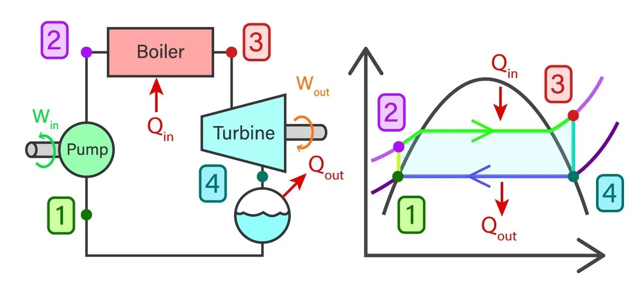
p-v, h-s and T-s plots:

Plotting with pressure-volume, enthalpy-entropy or Temperature-Entropy plots is a convenient of understanding any thermodynamic cycle. P-v diagram is mainly involved with the work interactions whereas the h-s and T-s plots reveal a great information as phase change, heat/work transfer etc over each thermodynamic process involved.

Types of Rankine Cycles and the thermal processes involved:

As discussed Rankine cycle comprises of four main thermodynamic processes out of which two are involving heat transfer as the Heat is generated by combustion in a boiler and the other two are involving the work transfer as in the turbine and a pump. Further, there are three types of Rankine cycles in practice. They are:

1) Saturated Steam Rankine cycle

2) Super heated Rankine cycle

3) Sub cooled Rankine cycle

The above are defined according to the quality of the steam.

The other rankine cycle classification is made as:

1) Rankine cycle with Reheat

2) Rankine cycle with Regeneration

3) Rankine cycle with both Reheat and Regeneration

Work interactions in Rankine cycle:

There are two types of work interactions in every Rankine cycle:

1) Work done through a pump

2) Work output from a turbine

Heat interactions in a Rankine Cycle:

On the similar lines as Work interaction, there are two Heat interactions inside a Rankine cycle as Heat produced by the combustion of the working fluid and also the second one will be the heat rejected to a Sink at much lower temperature (T₂) than the Source temperature (T₁).

h-s (Enthalpy-Entropy) diagram is conveniently used to analyse the Rankine cycle. Commercially a diagram called Mollier Chart is used which contains the x-coordinate(entropy) and the y-coordinate (enthalpy) which contains these values within the specified operating ranges. A sample of the Mollier diagram is as shown:

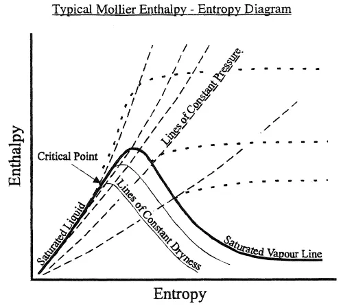
So, in the above case the limits in which a given type of Rankine cycle operates decides the efficiency and other parameters like net Work output and the net heat transfer from the cycle.

Usually all the required values that fall across a different class of the cycles are kept in a tabulated form called ‘steam tables’. These steam tables carry a large amount of data especially they throw the values near the required operating pressures (turbine inlet/exit in the case of pressure(where work done is important) or the heat/temperatures required to process the steam in the case of a boiler/condenser inlet/exit is of concern.

So, in order to calculate the required amount of net work output or the net heat transfer rate from the cycle what we require is the thermodynamic properties (enthalpy-enropy (or) temperature-entropy (or) pressure-volume)

So, these thermodynamic variables are to be retrieved at the specified temperatures and pressures (operating conditions).In this case ‘xsteam’ library is used to store the values required and with the help of a proper syntax, they may be retrieved from the data set at the required abscissa/ordinate whichever found suitable.

Thermodynamics of a complete Rankine Cycle:

From the schematic and the graphical representation of the whole Rankine cycle as discussed in the section Rankine cycle and Thermodynamics, the point of interest here which is appropriate use of the relevant ‘State’ properties of the working substance, Steam. Mainly required are the Pressure and Temperature and from which are deduced enthalpy, entropy, specific volume used to find out the required amount of work done or the net Heat transfer through the cycle.

In order to get the required properties at the necessary operating conditions, the intrinsic thermodynamic characteristic/fundamental thermodynamic principle of each process is to be understood clearly. Going in a sequential manner we observe these as follows:

1) Work done by pump(Process 1-2):

As we know that the function of a pump is to compress the liquid to the specified pressure, in a Rankine cycle, the pump works on the working substance Water and pressurizes it to the sufficient pressure to perform in the boiler. The work done by a pump is given by W = -v*(p₂-p₁).The negative sign is kept due to the compressive work done by pump on water.

Here the inlet enthalpy is the saturated liquid enthalpy at the inlet condition (pressure at inlet to the pump).

2) Work output from a turbine(Process 3-4)

The main important factor, the mechanical work output from a Turbine is to be understood as the expansion of the high temperature pressurized steam along the turbine. The process may be adiabatic process(Q=0) as the steam passes through the turbine at a very high velocity. Applying the steady flow energy equation, h_inlet = W_Turbine+h_exit

So, in this case we need to extract the enthalpies at the corresponding pressure/temperature by choosing whichever gives a consistent solution.

As in the case of a pump, we may observe here that the working substance is brought back to the liquid state after giving the sufficient work output from the turbine.

Note: Often, the fact that both the thermodynamic processes involving work in the pump or a turbine are isentropic processes is used to get the required thermodynamic quantities to be used in the appropriate equation.

3) Heat input into the cycle (Boiler) (Process 2-3)

Heat input into the cycle is calculated again by careful manipulation of the Steady flow energy equation. In the case of a boiler the work done is zero as the system being a constant volume system. So, the Steady flow energy equation throws back the Heat input as the change in enthalpy (kJ/kg) (a positive gain (h₃-h₂ ) as the heat is added into the system). Q = (h₃-h₂)

4) Heat interaction through a Condenser (Heat rejected) (Process 4-1)

The heat rejected through the condenser proves to be an isochoric (Constant volume) process similar to that of a thermodynamic process occurring in a boiler. So, the heat rejected is nothing but again the enthalpy change before entering the condenser and exiting the condenser. Q_rej = (h₄ –h₁ )

All these values are derived from the given ‘xsteam’ library by carefully ensuring the appropriate thermodynamic relations are applied without loss of any consistency.

Eg.: in the processes involving work, say that of Turbine, one of s3 or s4 is sufficient as these turnout to be equal as it is an isentropic process.

Finally the cycle efficiency is scrutinized for the following three cases in consistent with the ideal Carnot cycle but taking into account the practical considerations like Metallurgical considerations/Design of turbine etc:

1) Reducing the condenser pressure

2) increase the temperature of the Source (Boiler) (Metallurgical considerations)

3) Increasing the pressure in the boiler.

4) neglecting pump work.

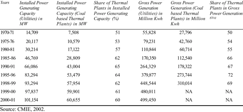
Indian Generation capacity:

%Basic Rankine cycle

%inlet pressure in the condenser

clear all

close all

clc

p4 = 0.05;

p1 = p4;%isobaric condenser process

%the maximum temperature

T3 = 400;

%the pressure in the boiler

p3 = 30;

p2= p3;%process 1-2 is isobaric heat addition inside the pressure vessel

%isentropic work done by the pump

v1= XSteam('vL_p',p1);

wp = -v1*(p2-p1)

%computation of Qaddn in pressure vessel

h1 = XSteam('hL_p',p1);

h2 = h1-wp;%steady flow energy equation

h3 = XSteam('h_pT',p3,T3);

Qaddn = (h3 - h2)

%Computation of the work in the turbine

s3 = XSteam('s_pT',p3,T3);

s4 = s3;

h4 = XSteam('h_ps',p4,s4);

wT = (h3 - h4)

%computation of the quality of the steam at the exit of the turbine

x4 = XSteam('x_ps',p4,s4)

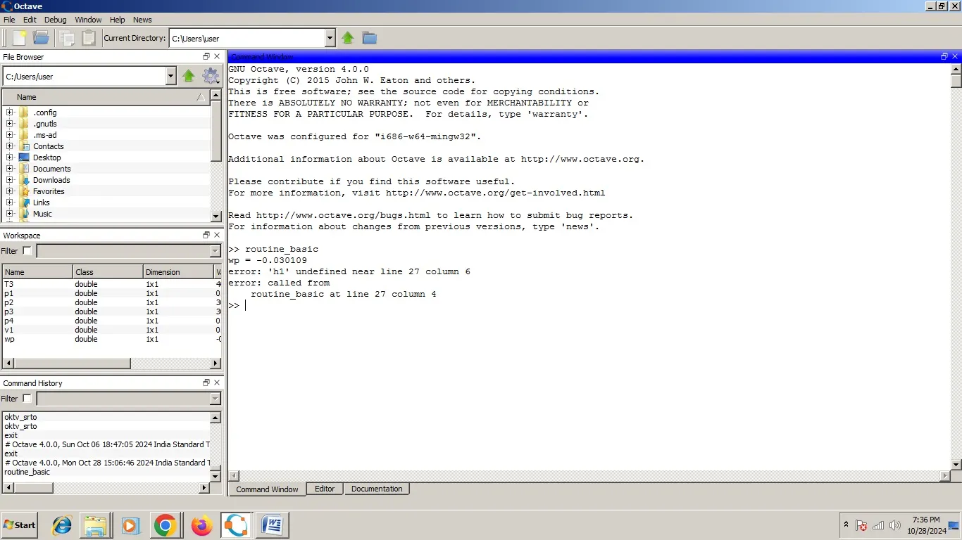
the following error was encountered while we tried to execute the program:

it is later corrected by following proper syntax while calling the function.

We could obtain the following output when the above routine was properly executed with the details of the specified power plant operating conditions:

Turbine inlet temperature = 400 deg.C

Turbine Inlet pressure = 30 bars

Condenser inlet pressure = 0.04 bar = Turbine outlet pressure

All through the calculations, the net work output will be the pump work subtracted from total Turbine work

the required result obtained is as follows:

net work output = 1120.9 kJ/kg

back work ratio = 0.000026863

It would be wise to observe that whole functioning and efficiency of the above cycle is interdependent on different type of values each of the above set parameters/operating conditions. So, a feasible solution looks for a consistency in terms of the thermodynamics of the cycle reflected mainly in the thermodynamic relations.

A careful manipulation of the above values (only one value at a time, others remaining constant) is considered as follows as a Research interest:

The following three cases may be considered considering the practical considerations which take into account many interesting equipment like Feed Water Heater, Economiser, Super heater etc.

Case1:

Changing the condenser pressure (working along the direction of the 'Sink' operating conditions)

pressure at the exit of the turbine and the inlet of the condenser = 0.1 bar

Temperature inside the pressure vessel = 400 deg.C

Pressure inside the vessel above = 30 bar

taking above values as input, we have the following result:

where we have work output as:

1038.6 kJ/kg and

back_work_ratio = 0.000029084

In this case as the Sink conditions vary, increasing the operating pressure in the same, the net work output is reduced.

Case 2:

Observing the changes with the change in the Operating temperature of the boiler

So, the following parameters may be considered

pressure at the inlet of condenser/exit of turbine = 0.04 bar

temperature inside the pressure vessel = 600 deg.C (this is taken with reference to the metallurgical considerations of the material)

pressure inside the same = 30 bar

by running the simulator, we get the following result

as a note, we should observe here that we are increasing the temperature at which heat enters the system or we are increasing the 'Source' temperature and we can easily say that the Work output is obviously increased which may be inferred even from the T-s diagram of the Rankine cycle (increasing the upper limit increases the distance (height) between the Source temperature and the Sink temperature.

The same argument applies in the case of decreasing the condenser inlet pressure which also has the same effect on the net work output as the distance between the two increases.

In practice, it may be noted that in order to get an increased work output, the second case which is changing the condenser pressure is ideally suited keeping in view the temperature limits which are an important Metallurgical consideration is to be borne in mind while taking any decision.

the following result is obtained for Case 2:

net work output = 1420.07 kj/kg

back work ratio = 0.000021183

Case 3:

Observing the changes in the output by varying the operating pressure of the process in the boiler

the following parameters may similarly be considered:

Pressure at the exit of turbine and the inlet of Condenser: 0.04 bar

Operating Temperature inside the boiler = 400 deg.C

Pressure inside the pressure vessel = 50 bar

the point of interest the pressure rise inside the pressure vessel is a fact to observed considering the design considerations. Considering it as shells and plates, the maximum stress criteria while designing a pressure vessel is to be considered. The folowing figure depicts clearly the elastic deformation observed in a pressure vessel.

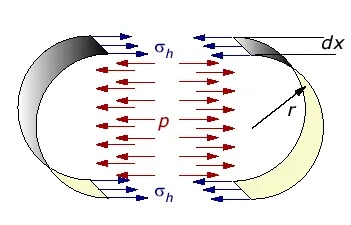
formulae 'pr/t' and 'pr/2t' (r-radius of the pressure vessel and t- thickness of the pressure vessel) may be applied to get the two principal stresses while designing a Factor of Safety for a pressure vessel for safe design.

We have the following output in the current case:

net work output = 1194.3 kJ/kg

back_work_ratio = 0.000042002

Case 4:

Neglecting the work done by a pump in all the above cases concerning all the above power plant utility cases:

the following table summarizes the values of both, the turbine work output and the work done by that of a pump.

	Turbine Work (kJ/kg)	Pump Work (kJ/kg)(mod value)
Case 1	1038.06	0.0302
Case 2	1420.1	0.0301
Case 3	1194.3	0.0502

So, the above table gives an insight how we can neglect the pump work which is less significant or of low order of magnitude than that done by a turbine.

Conclusion: Rankine Cycle analysis by varying state variables is complete.