Week 4.1 - Solving second order ODEs

Question:

1. write a MATLAB program that solves the following ODE which represents the equation of motion of a simple pendulum with damping.

2. Simulate the pendulum motion with given parameters.

Given:

g = acceleration due to gravity = 9.81 m/s2

L = length of the pendulum = 1 metre

m = mass of the ball = 1 Kg

b = damping coefficient = 0.05

To simulate the motion of the pendulum,

Time span = 0 -20 s

Angular displacement = 0 at t = 0

Angular velocity = 3rad/s at t = 0

Solution:

In Engineering, Ordinary Differential Equation (ODE) is used to describe the transient behaviour of a system. A simple example is a pendulum. A simple pendulum consists of a ball of mass ‘m’ hanging from a string of length ‘L’ fixed at a pivot point P. When displaced to an initial angle and released, the pendulum will swing back and forth with periodic motion.

By applying Newton’s second law for rotational systems, the equation of motion of pendulum is obtained which is known as ODE.

In MATLAB, ODE45 solver needs a simple differential equation to solve higher order differential equation. Since, it is a second order ODE we need to break it into first order ODE.

Hence,

Consider,

θ = θ1 ------ (1)

dθ/dt = dθ1/dt = θ2 ------(2)

d2θ/dt2 = dθ2/dt -------(3)

Putting the above values stepwise in the ODE we get,

dθ2/dt = -(b/m) * θ2 – (g/l) * sinθ

Now, we have the first order ODE which can be written in the matrix form as,

From the above considerations, equations and representation of the equation in matrix form, we can create a program code to solve the equation.

For this, a function code solving the ODE is created which would be called in the main code.

FUNCTION CODE

function [dtheta_dt] = ode_eqn(t,theta,b,g,l,m)

       

% Formulating second order ODE into simple ODE

        theta1 = theta(1);

        theta2 = theta(2);

        dtheta1_dt = theta2;

        dtheta2_dt = -(b/m)*theta2 - (g/l)*sin(theta1);

        dtheta_dt = [dtheta1_dt ; dtheta2_dt];

end

MAIN CODE

clear all

close all

clc

 

%Inputs

l = 1;

m = 1;

b = 0.05;

g = 9.81;

 

%Initial condition

theta_0 = [0;3];

 

%Time span for pendulum simulation

t_span = linspace (0,20,200);

 

%solve ODE

[t, results] = ode45(@(t,theta) ode_eqn(t,theta,b,g,l,m),t_span,theta_0);

 

%Plotting the graph

figure(1)

plot(t,results(:,1))    % time vs Angular displacement

hold on

plot(t,results(:,2))    % time vs Angular velocity

xlabel('Time')

ylabel('Plot')

legend("Angular displacement","Angular velocity")

 

% Using for loop to simulate the pendulum

ct = 1;

for i = 1:length(results(:,1))

    X0 = 0;

    Y0 = 0;            % position of pivot

   

    X1 = l*sin(results(i,1));

    Y1 = -l*cos(results(i,1));    % positions of the bob

 

    % Plotting the animation

    figure(2)

    plot([-1 1],[0 0],'linewidth',7, 'Color',"black") % base

    hold on

    plot([X0 X1],[Y0 Y1],'linewidth',1, 'Color','g')  % string

    hold on

    plot(X1,Y1,'o','markersize',10,'markerfacecolor','b') % bob

    axis([-2 2 -2 2])

    pause(0.03)

    hold off

 

    M(ct) = getframe(gcf);   % Storing all the images in variable M

    ct = ct+1;

end

 

% Creating movie file of the animation

movie(M)

videofile = VideoWriter('pendulum.avi','Uncompressed AVI');

open(videofile)

writeVideo(videofile,M)

close(videofile)

 

EXPLAINATION OF CODE:

• A function code named as ode_eqn is created using ‘function’ command in which the second order ODE is converted to simple ODE.
• For the main code, the given inputs (l,m,b,g) are inserted. At theta = 0 the angular displacement and angular velocity are 0 and 3 respectively. The time span (t_span) of 20 seconds with 200 iterations is provided for the simulation of pendulum using linspace command.
• In the next step, the MATLAB inbuilt ODE solver command ODE45 is used and for that, the created function is called. As it is a second order ODE the variable ‘results’ will store two sets of values of angular displacement and angular velocity.
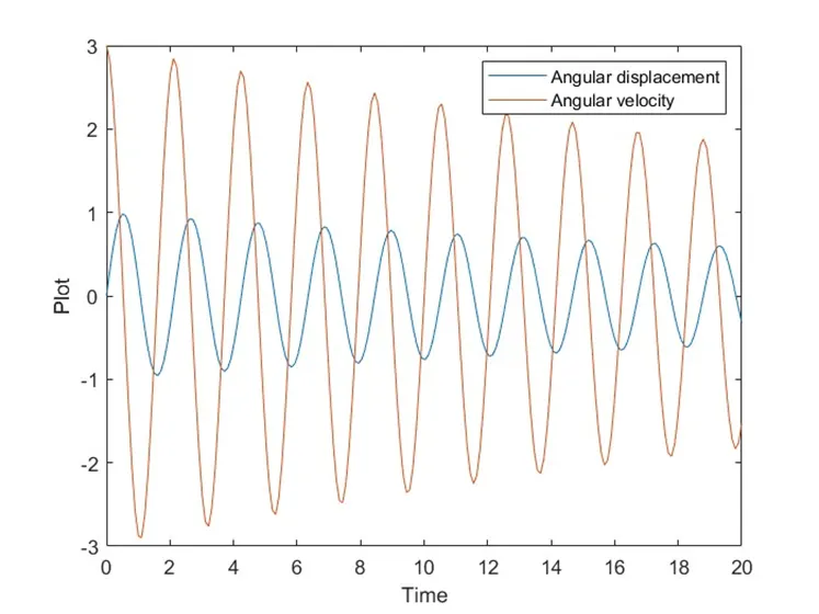
• For the graphical representation of the motion of simple pendulum, plot command is used for plotting the values of angular displacement and angular velocity extracted from variable ‘results’.
• For the simulation of pendulum, we need to provide the different points of angular displacement. Hence, for command is used. The point for pivot x0, y0 is determined and position of the bob is calculated using trigonometry.
• To construct the simulation, plot command is used wherein,

1. The base/wall is plotted with colour black.
2. The string is plotted with colour green.
3. The bob is plotted with colour blue.

• Axes limits and a pause of 0.03s is given for a smooth simulation.
• All the pictures of iterations are stored in a variable M to create a movie of the simulation.
• By using Movie command a video file of the simulation is created. The videofile command saves the video with a given name.

OUTPUT PLOT:

CONCLUSION:

A second order ODE from a motion of a simple pendulum is solved using MATLAB code and the motion of the pendulum is graphically presented with also creating a simulation of the motion.

Video Link:

https://drive.google.com/file/d/1mu6sVi8Xuwo-3lpG65q_i2qFltFXK6oe/view?usp=sharing