Week 4.1: Project - Steady state simulation of flow over a throttle body

Throttling Process:

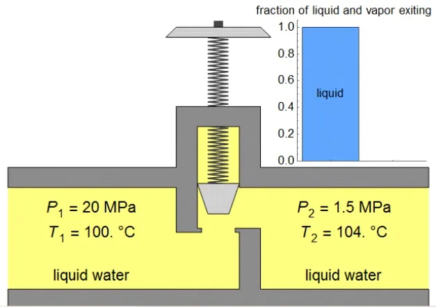
A process in which the flow of the fluid partially restricted by any how that cause a high pressure drop in the fluid. The idea is that you throttle down the pressure, the speed of the flow increases, the temperature drops, but reversibly in the thermodynamic sense.

How to perform a throttling process?

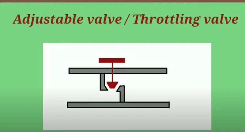
• By an adjustable valve
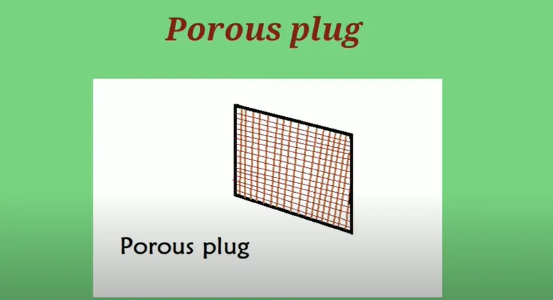
• By a porous plug
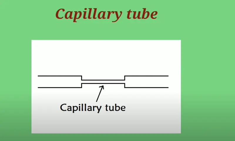
• A capillary tube

Adjustable Valve

Technically, a throttle valve with a metaphorical capitol T is designed so as to have little entropy loss.

Porous Plug

Capillary Tube

Throtlle Body:

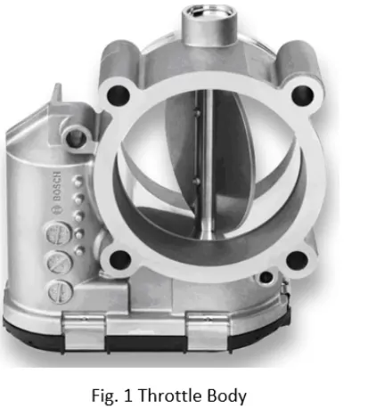
A throttle body is essentially a large air valve that lies between the intake manifold and the air intake pipe. An engine has a throtlle body which bolts to the intake manifolds plenum( the large air cavity in the centre). It controlles air flow into the engine, a crutual fector for controlling the engine's air fuel ratio. Throtlle bodies comes in several shapes, sizes and configerations. They can perform several tasks other than air meetering duties.

Throttle bodies usually use butterfly valves. Butterfly valve is a plate that pivots about an axis. A butterfly valve has the disc that blocks the flow rotating on the stem of the valve. The stem bisects the plane of the disc.

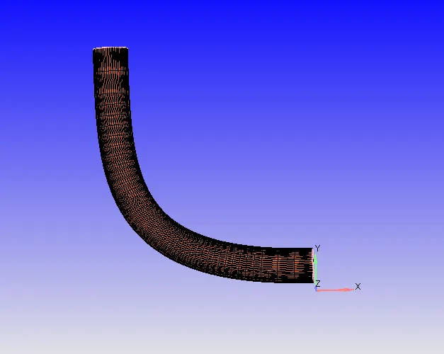
View of Geometry

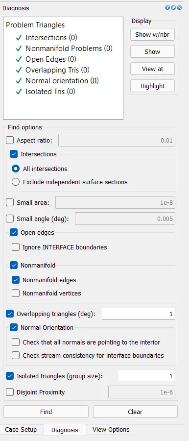
Run Diagnosis

• To ensure that the geometry is clean, click Diagnosis tab and click on Find

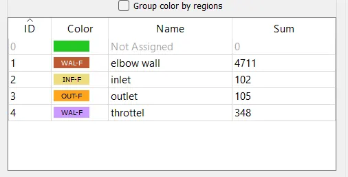
Boundry Flagging

• Add the boundaries by clicking create multiple boubdaries to create all boundaries at a once and name them like Elbow_wall, Throttle_valve, top, inlet and outlet by selecting the respective triangles.

• Then click Normal Toggle option and click any one of the triangle which shows the normal that is opposite to the direction of fluid flow and click Apply.

CASE SETUP

• In order to begin the case-setup, click on the case-setup and click begin case-setup and click Time based, since it is not a crank angle based like IC engines or Pumps but a steady-state channel flow setup.
• Then click on Materials and select Air to be predefined mixtures.
• Then open the Gas simulation and Global transport parameters and retain the default setting. And also retain the same setting for the species and Reaction mechanism.
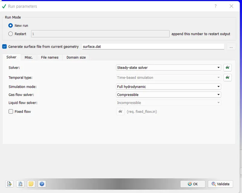
• Then click on the Run Parameter under the Simulation Parameter and choose the Steady state solver under the solver tab and then choose the Full Hydrodynmic under the simulation mode. And then choose the Compressible under the Gas flow solver.
• In the Miscellaneous tab, check the steady state monitor and uncheck the use shared memory because of we are running a steady state simulation flow here.
• Then click on the Steady-state monitor, click add config. And click Add to add the variables that needs to be monitored.

Run Paremeter

Steady Stata Monitor

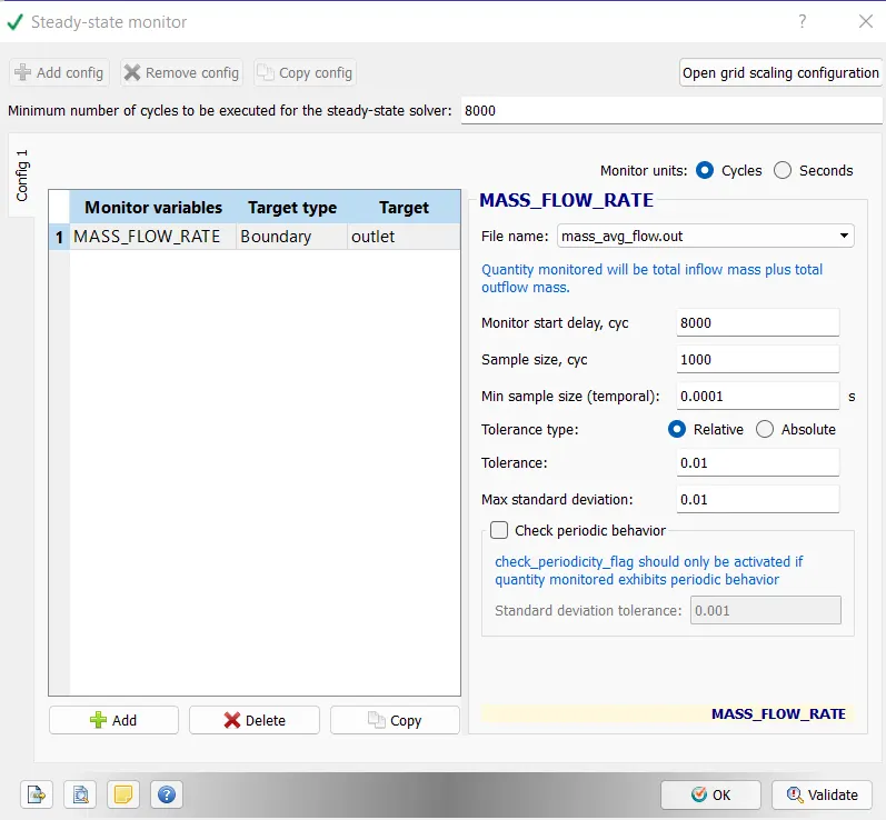
• The monitor start display is a parameter that ensures that the simulaion runs for a certain number of cycles before the variable can be monitored. This is especially useful in transient simulations when you want the solution to run for a particular amount of time before checking for convergence, if the steady state results are also required.
• Sample size denotes the number of cycles or seconds over which the variable is checked to see if the solution has converged. The solution is said to be converge when the average change over multiples iterations is less than the tolerance value. The tolerance value can be changed based on the problem and level of accuracy required.
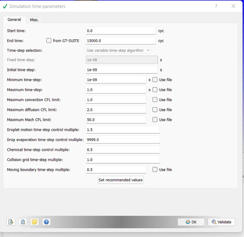
• In the simulation time parameter do the following changes.

Simulation Time Parameter

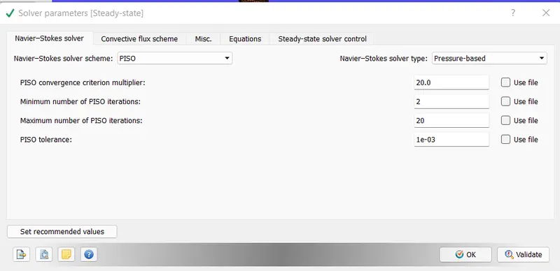
Solver Parameter

• In the solver time parameter, we only choose the pressure based solver and retain the remaining setting.

Boundry Conditions

Inlet:

• At the inlet boundary we specify the inlet pressure 150000 Pa and select the predefined mixture as a Air which contains N2 as a 77% and O2 as 23%. And select the temperature to be specified of 300K.

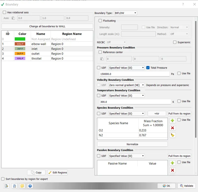
Outlet:

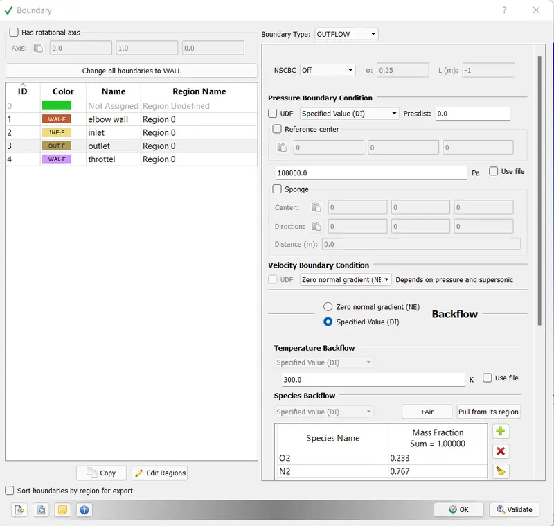
• At the outlet boundary, we specify the 100000 Pa pressure.

Elbow Wall

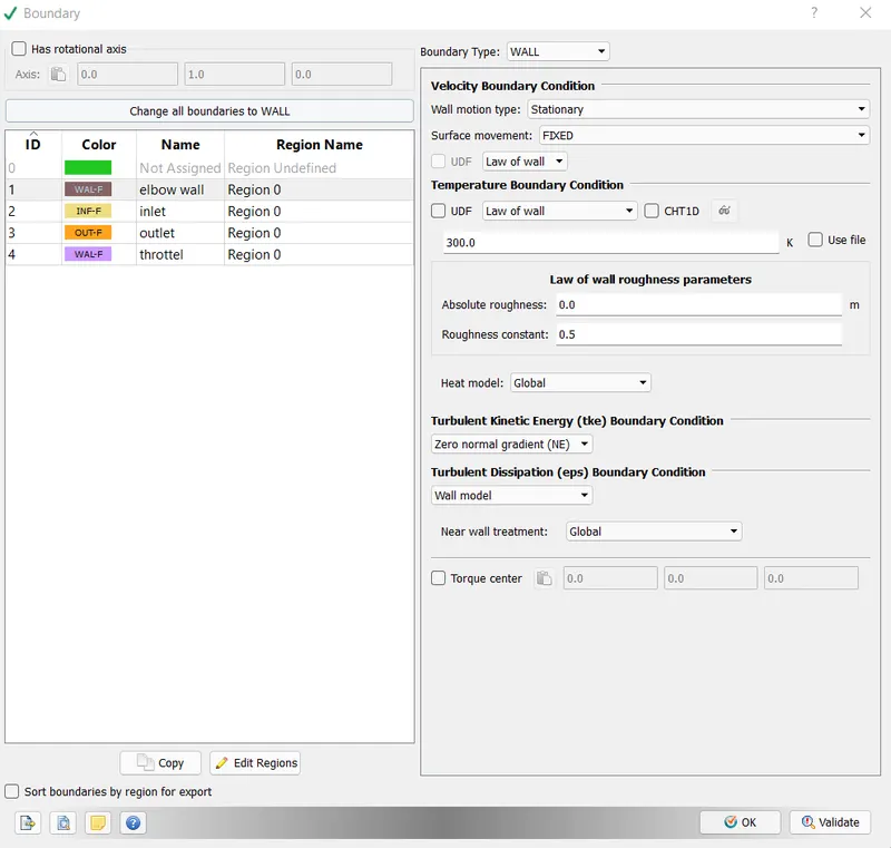
At the Elbow , we are taken the wall boundary condition

Throtlle:

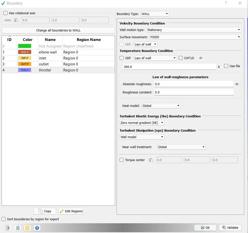
At Throttle valve , we are taken the wall boundary condition

Regions and initialization

• In Regions and Initializations, click Add as Region 0.

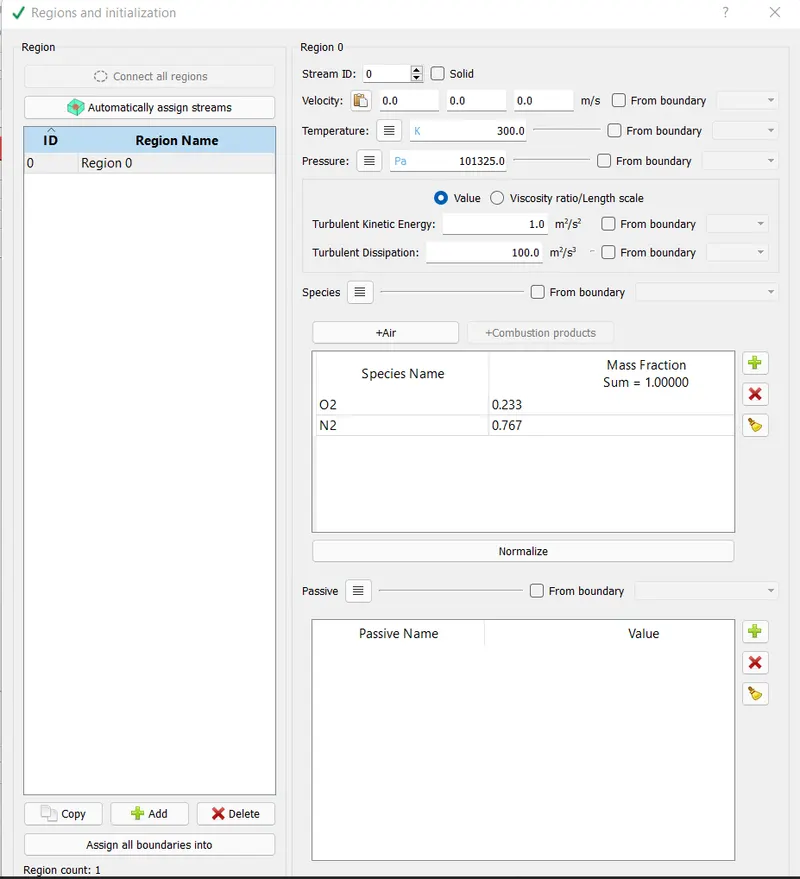
• Goto Physical Models and check the Turbulence Modelling and choose the RNG/k-epsilon model.
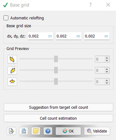
• Then in the grid control, the mesh size that want to be created is in meters.
• For Output files, Time inter for writing 3D output files is 100 cycles which is the time interval between the one and another output file that get dumped in output files successively and the maximum no. of restart files that saved is 3 which is a factor of safety and click ok.

Base Grid

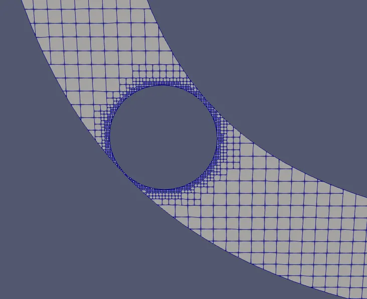
Fixed Embedding

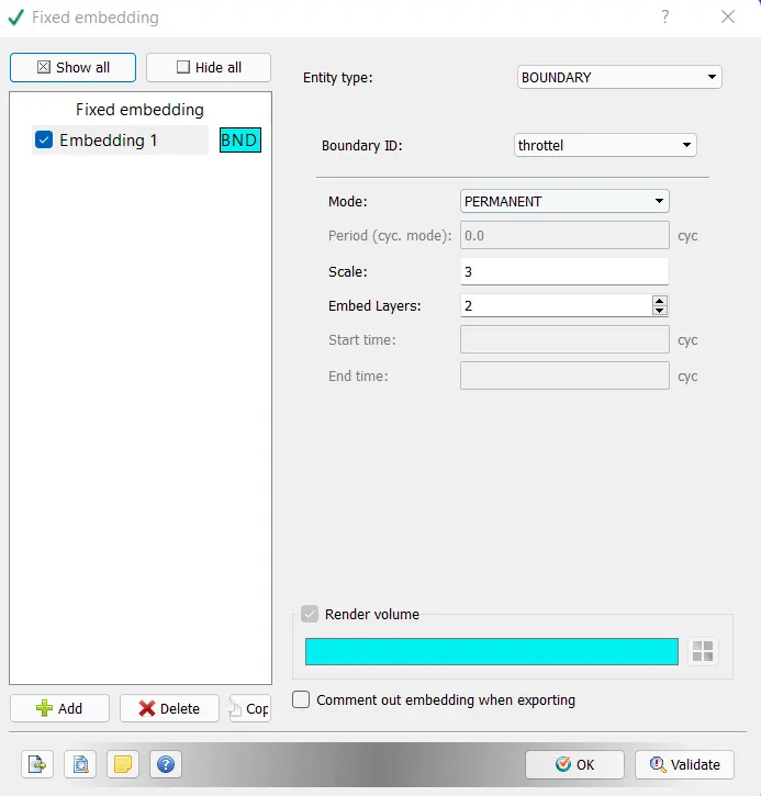
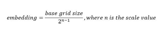
Here n=3, base grid size =0.002

embeddind =`0.002/2^(3-1)`

embedding=`0.002/4`

embedding =0.0005

so near the throttle the two layers will be formed with mesh 0.0005

Output Files

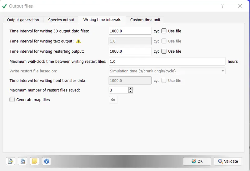
• At the end all the inputs files have to be exported:

File -->Export-->Export input filesq

Analyzing the plots in Converge CFD

Presurre

Total Presuure at inlet and outlet

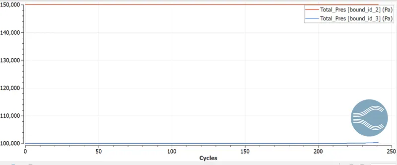
Boundry id_2 is inlet and Boundry id_3 is outlet

• Fluid flows due to pressure difference. so at inlet we have given the value of total pressure 150000 Pa and total pressure at outlet is 100000 Pa.

Pressure at inlet

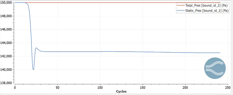
Boundry id_2 is inlet and Boundry id_3 is outlet

• At the inlet plot of pressure, we observe that initially total and static pressure is same which is 150,000 Pa. And we also know that total pressure = static pressure+dynamic pressure and initially dynamic pressure is zero.
• As the cycles going on the static pressure is going to decrease due to increase in dynamic pressure.
• After 13 cycles the static pressure is going to decrease rapidly due to fastly movement of fluid.

Pressure at outlet

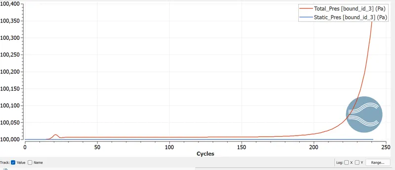
Boundry id_2 is inlet and Boundry id_3 is outlet

• Finally at the outlet the static pressure reaches to 100,000 Pa and the value of the total pressure is increases due to increase in dynamic pressure.

Velocity

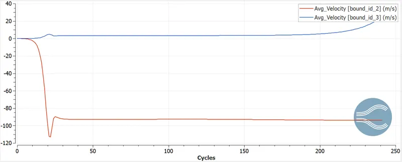
Boundry id_2 is inlet and Boundry id_3 is outlet

• In the above velocity plot, we easily observe that at the inlet velocity is decreases rapidly after 8 cycles due to increase in pressure at inlet.
• At the outlet, we observe that the velocity is increasing due decrease in pressure.
• At inlet the velocity is decreased and reaches to -92.79 m/s and at the outlet the velocity is increased and reaches to 3.3 m/s.
• It occurs since the pressure is inversely proportional to the velocity.

Mass Flow rate at inlet and outlet

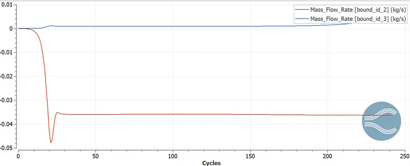
Boundry id_2 is inlet and Boundry id_3 is outlet

• Mass flow rate is defined as the mass of substance which passes per unit time.
• Here in the mass flow rate at the outlet there is a jump at x=20 cycles
• Then Finally at the inlet the value of the mass flow rate is -0.0359367 (kg/s) aprox and at the outlet the value of mass flow rate is 0.00905313 (kg/s)
• negative sign shows that the mass is going inside and the positive sign shows that the mass is going outside.

Total Cell Count

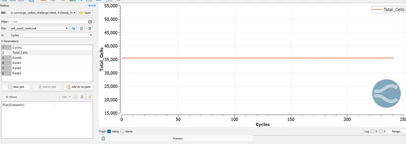
• Since i have used the 4 processors and the total cell count is 35,518.

Load on 4 processors

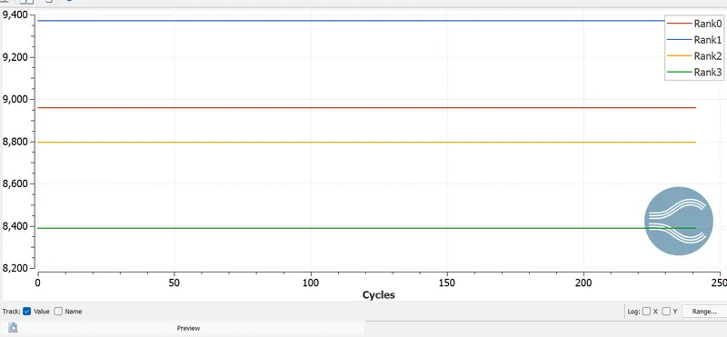
• Processor 1 is handling 8960 cells.
• Processor 2 is handling 9372 cells.
• Processor 3 is handling 8797 cells.
• Processor 4 is handling 8389 cells.
• 8960+9372+8797+8389=35518 (total cell count)

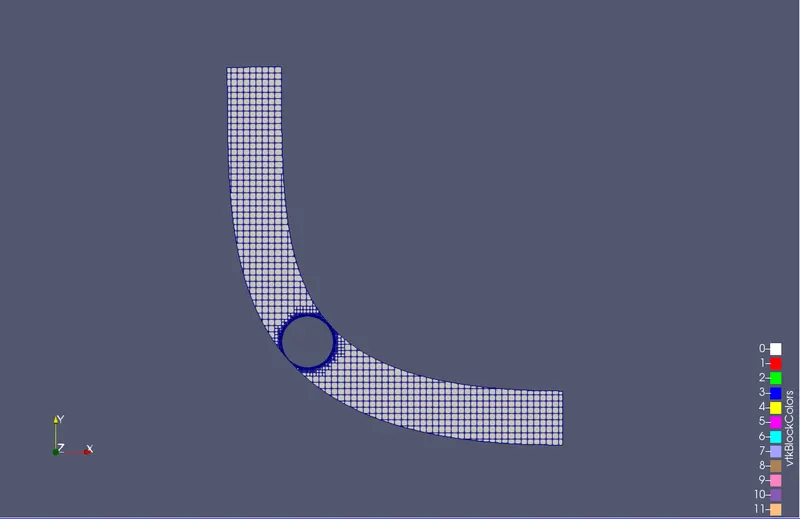
Mesh( Surface with edges)

Fine mesh near throttle

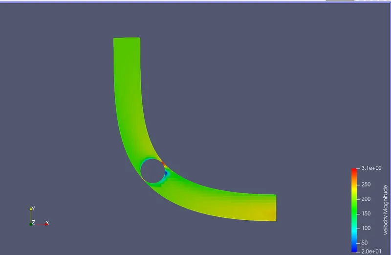
Velocity Contour

Observation from plot

In the above plot we can easily observe the three regions which we can see

• Top left blue colour region shows that the velocity decreases as it is near about about the throttle.
• Red region shows the high velocity which is approximately 310 m/s. This is the narrow path where the fluid passses and that's why velocity is increases.
• And bottom right blue region shows the recirculation region. Flow separation is also occuring here, eddies are formed here and velocity drops as low as 20 m/s.

Velocity Vectors

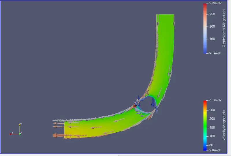
• Velocity vectors ensure that flow moves in right direction i.e from inflow to out flow boundry.

Pressure contour

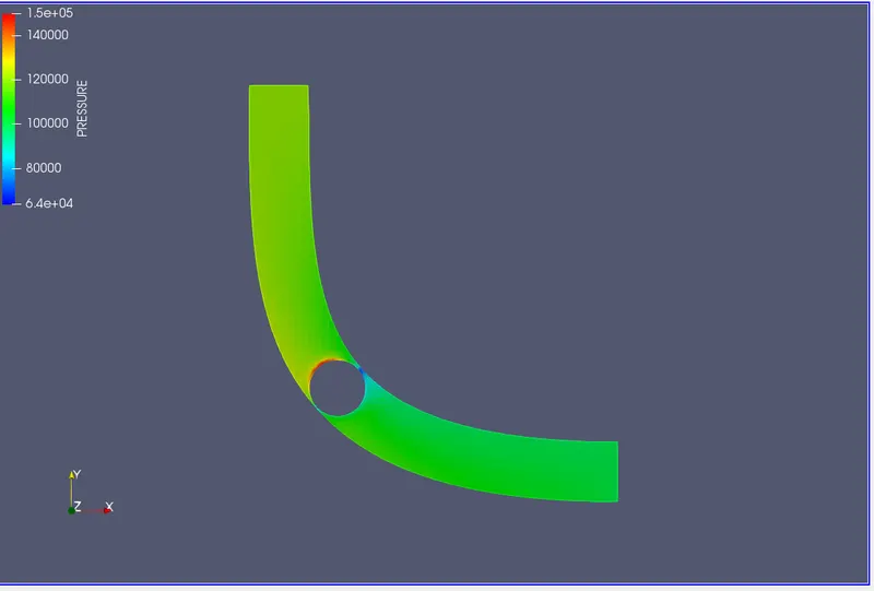
Observation from plot

In the above plot we can easily observe the two regions which we can see

• Red region shows the high pressure which is between 1.4 to 1.5 bar.
• And blue region shows the low pressure. The pressure drop because the flow is constricted.

Pressure contour for throttle

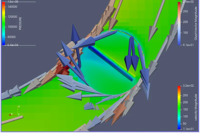
• when flow encounter the throttle, pressure is bit high. then we have low pressure rejions because there the flow is seperted.
• low pressure indicates drop in static pressure.

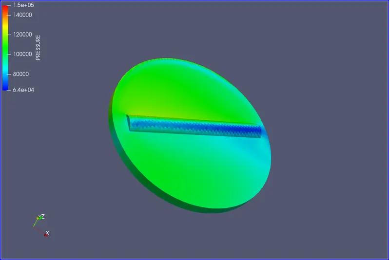
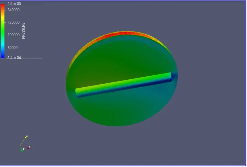
• There is some flow through the side as shown in the figure below because the throttle is not perfectly sealing the channal

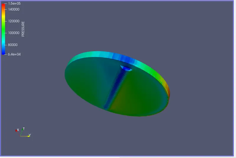
• On the throttle, we also observe the two region which is red and blue. Red colour shows the high pressure region and blue colour shows the low pressure region. In high pressure region fluid impose the pressure on the throttle as it flows over the throttle body.
• And the low pressure region(blue region) is due to the flow separation happening near the axis of rotation of the throttle.