Week 1: Channel flow simulation using CONVERGE CFD
Channel Flow Simulation using Converge Software
Aim:
The main objective of this challenge is to simulate the simple 2D channel flow in converge CFD software. The simulation is done using three different meshes and compared the plots of velocity, pressure, total cell count and mass flow rate in all the meshes.
Introduction:
Fluid flow with in the well bounded structure whose volume is completely occopied such that flow accross the crossectional area takes place due to pressure gradient can be cherectorised as internal flow. Transport of oil and gass distributed over long networks of piping conections, hot and cold water flow pumped to taps in homes are some comertial and industrial of the examples of internal flow
Steady Flow Between Paralell Plates
Flow assumptions:
1) Incompressible flow i.e `rho` constant
2) Viscosity is assumed constant. i.e μ is constant
3) Fully developed flow ∂u/∂x=0
4) Steady flow
5) In x direction. u ≠0, v=0, w=0
flow between two paralell, stationary plates i.e -∞<x<∞ ( in general problem we are taking this)
spacing between them is finite 0≤y≤2a
6) 2 dimensional flow. u=u(x,y). means vilocity also varries along y direction. infact vilocity at centre will be maximum.
7) Body force is neglected.
8) Boundry layer flow. viscosity effects are significant in the boundry layer region.
Governing Equations:
1) Continuty Equation
`(partial rho)/(partial t)+ nabla.(rho v)=0`
2) Momentum equation
`rho((partialv)/(partialt)+v.nabla)=rho beta-nabla p+mu nabla^2v`
Boundry conditions:
no slip condition
u=0 at y=0 (lower plate)
u=0 at y= 2a (upper plate)
Governing Equations In Component form:
Continuty equation in component form
`nabla.v=0`
`(partial u)/(partial x)+cancel(partial v)/(partial y)+cancel(partial w)/(partial z)=0`
`(partial u)/(partial x)=0`
Momentum equation in component form
X component
`rho(u(partialu)/(partial x)+v(cancelpartialu)/(partial y)+w(cancelpartialu)/(partial z))=-(partial p) /(partialx)+mu(partial^2u)/(partial^2x)+(partial^2u)/(partial^2y)+(cancelpartial^2u)/(partial^2z` eq2
Y component
`rho(u(cancelpartialv)/(partial x)+cancelv(partialv)/(partial y)+cancelw(partialv)/(partial z))=-(partial p) /(partialy)+mu(cancelpartial^2v)/(cancelpartial^2x)+(cancelpartial^2v)/(partial^2y)+(cancelpartial^2v)/(partial^2z` eq3
Z component
`rho(u(partialw)/(partial x)+v(cancelpartialw)/(partial y)+w(cancelpartialw)/(partial z))=-(partial p) /(partialz)+mu(cancelpartial^2w)/(partial^2x)+(cancelpartial^2w)/(partial^2y)+(cancelpartial^2w)/(partial^2z` eq4
by eq 3 and eq 4 we get
`(partialp)/(partialy)=0 and (partialp)/(partialz)=0`
so pressure is constant in y and z direction
eq 2 implies
`-(partialp)/(partialx)+mu (partial^2u)/(partialy^2)=0`
or
`-(dp)/dx+mu (d^2u)/dy^2=0`
`(d^2u)/dy^2=1/mu (dp)/dx` eq5
we have to solve eq5 subject to theboundry conditions. To discuss the problem of steady, imcompresible, fully developed flow between two infinite paralell stationary plates. Integrate eq 5
`(du)/dy=1/mu(dp)/dx y+c1`
again integrating we get
`u(y)=1/mu(dp)/dx y^2/2+c1y+c2` eq6
To find c1and c2 we use given boundry conditions
put u=0 at y=0 in eq 6 we get
c2=0
put u=0 at y=2a in eq 6 we get
`1/mu (dp)/dx(4a^2)/2+c1(2a)+0=0`
`c1=-a/mu(dp)/dx`
Using values of c1 and c2, eq 6 gets the form
`u(y)=1/mu(dp)/dx (y^2)/2-a/mu(dp)/dx y` eq7
this is the expression for velocity of the fluid between two paralel plates'
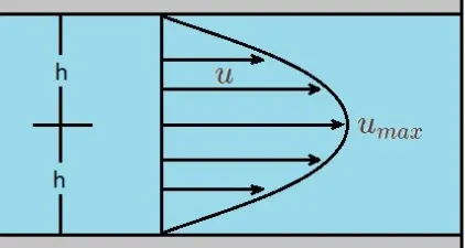
Velocity Profile:
velocity profile will be parabolic in nature
Volume Flow Rate:
`Q=int_(y=0)^(2a) udy`
put value of u we get
`Q=int_0^(2a)(1/mu(dp)/dxy^2/2-a/mu(dp)/dxy)dy`
`Q=-2/3a^3/mu (dp)/dx`
Average Velocity
`overlinev=Q/A=Q/(2a)`
`overlinev=-(2/3a^3/mu(dp)/dx)/(2a)`
`overlinev=a^2/(3mu)(dp)/dx`
Point of maximum velocity:
`u(y)=1/mu(dp)/dxy^2/2-a/mu(dp)/dxy`
`u(y)=1/mu(dp)/dx(y^2/2-ay)`
since velocity will be maximum at y=a. The above equation becomes
`u(y)=1/mu(dp)/dx(a^2/2-a^2)`
`u(y)=-a^2/(2mu)(dp)/dx`
Vertex:
`u(y)=1/mu(dp)/dx(y^2/2-ay)`
`2u(y)=1/mu(dp)/dx(y^2-2ay)`
`2u(y)=1/mu(dp)/dx(y^2-2ya+a^2-a^2)`
`2u(y)=1/mu(dp)/dx((y-a)^2-a^2)`
`(2u(y))/((dp)/dx)mu+a^2=(y-a)^2`
`(2mu)/((dp)/dx)(u(y)+a^2/(2mu)(dp)/dx)=(y-a)^2`
For vertex x=0 ,y=0 but here `X=u+a^2/2mu(dp)/dx and Y=y-a`
so vertex is `(a, -a^2/(2mu)(dp)/dx)`
Geometry Preparation:
- First of all open the converge and launch the new project.
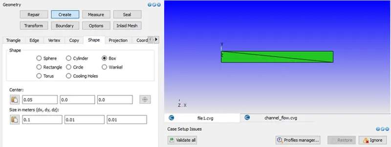
- Then in the Geometry box click on create then click on shape and then click on Box. After that enter the dimension of the channel case and then click on create.
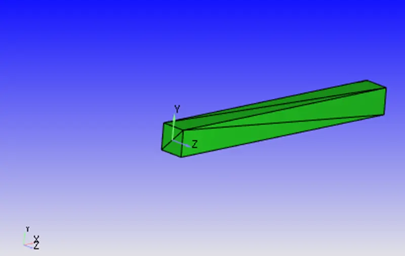
- 3D view of the geometry.
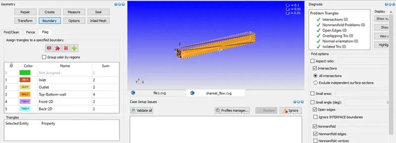
- To create a boundary surface make sure that cursor picked the triangle.
- Then select the boundary, in the flag tab, click + to add the boundaries.
- Add the boundaries by clicking create multiple boubdaries to create all boundaries at a once and name them like inlet, outlet, top and bottom walls, front 2D and back 2D by selecting the respective triangles and click.
- Then click Nomal Toggle option and click any one of the triangle which shows the normal that is opposite to the direction of fluid flow and click Apply.
- Then click on options and under the tab of Visibility, click Geometry Bounding box to create boundary line across geometry.
- To ensure that the geometry is clean, click Diagnosis tab and click on Find.
- All the parameters that got checked shows the green colour tick mark.
Case-setup
- In order to begin the case-setup, click on the case-setup and click begin case-setup and click Time based, since it is not a crank angle based like IC engines or Pumps but a steady-state channel flow setup.
- Then click on Materials, uncheck the Reaction Mechanism since there is no chemical reaction takes place and select Air to be predefined mixtures.
- Since there is no role of turbulence here, click Physical Models and uncheck the Turbulence Modelling.
- Then open the Gas simulation and Global transport parameters and retain the default setting.
- Then click on Species and add the N2 and O2.
- Then click on the Run Parameter under the Simulation Parameter and choose the Steady state solver under the solver tab and then choose the Full Hydrodynmic under the simulation mode. And then choose the Compressible under the Gas flow solver.
- In the Miscellaneous tab, check the steady state monitor and uncheck the use shared memory because of we are running a steady state simulation flow here.
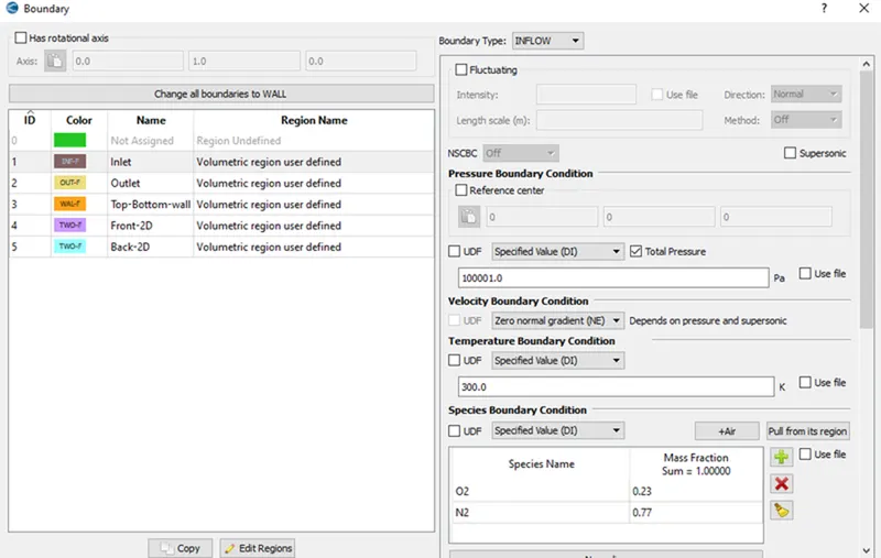
- At the inlet boundary we specify the inlet pressure 100001 Pa and select the predefined mixture as a Air which contains N2 as a 77% and O2 as 23%. And select the temperature to be specified of 300K.
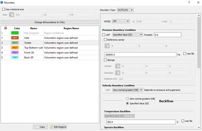
- At the outlet boundary, we specify the 100000 Pa pressure.
- At the top and bottom walls, we are taken the no-slip condition.
- At the front and back boundary, we are taking the boundary type as a Two_D. To run a two dimensional simulation in converge, use the TWO-D boundary type. The TWO-D boundary is available only for non-moving and non-spray cases. To set up a two-dimensional case in CONVERGE, create a three-dimensional surface
including two identical, parallel boundaries and set their boundary type to TWO_D. Note that the normal vectors of the corresponding TWO_D boundaries must be in the z direction (positive or negative). Thus, the two-dimensional flow occurs in the xy plane. Ensure that in the surface geometry, no vertices exist in the thickness between the parallel TWO_D boundaries. - Then click on the Steady-state monitor, click add config. And click Add to add the variables that needs to be monitored.
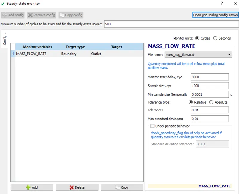
- The monitor start display is a parameter that ensures that the simulaion runs for a certain number of cycles befoe the variable can be monitored. This is especially useful in transient simulations when you want the solution to run for a particular amount of time before checking for convergence, if the steady state results are also reuired.
- Sample size denotes the number of cycles or seconds over which the variable is checked to see if the solution has converged. The solution is said to be converge when the average change over multiples iterations is less than the tolerance value. The tolerance value can be changed based on the problem and level of accuracy required.
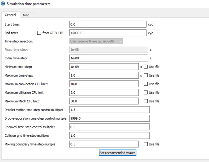
- In the simulation time parameter do the following changes.
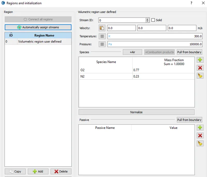
- In Regions and Initializations, click Add as Region 0 and set pressure as 100000 Pa since the flow should not reversed and click Air as its species.
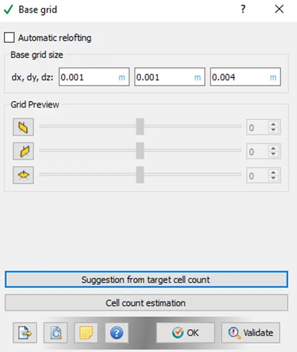
- Then in the grid control, the mesh size that want to be created is in meters.
- Then in the post variable selection, click on species/passive, check the mass fraction and add the N2 and O2.
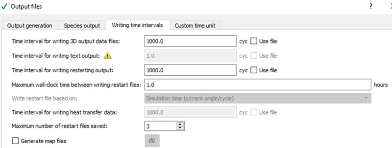
- For Output files, Time inter for writing 3D output files is 100 cycles which is the time interval between the one and another output file that get dumped in output files successively and the maximum no. of restart files that saved is 3 which is a factor of safety and click ok.
- Now when we click on validate all options for validating, we got the errors.
- To Resolve these errors, we go to Regions and initializations and rename the region 0 to Voulmetric region user defined and then go Boundary to assign this region to all the boundaries we have ceated since the error is not assigning the region for those.
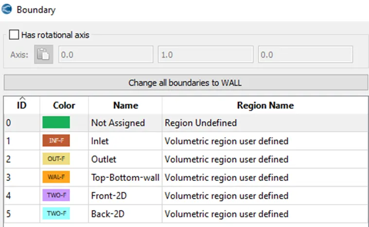
- And then click on validate all again and there will be no errors and the validation has been successfully complete.
- At the end all the inputs files have to be exported:
File -->Export-->Export input files
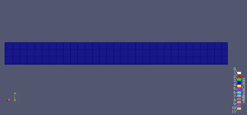
Mesh for the size 2e-04:
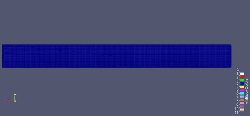
Mesh for the size 1.5e-04:
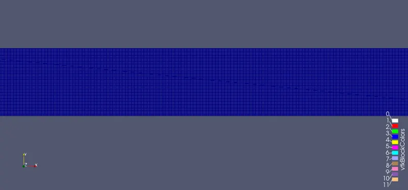
Mesh for the size 1e-04:
Analyzing the plots in Converge CFD
- For Mesh size 2e-04
Velocity Plot
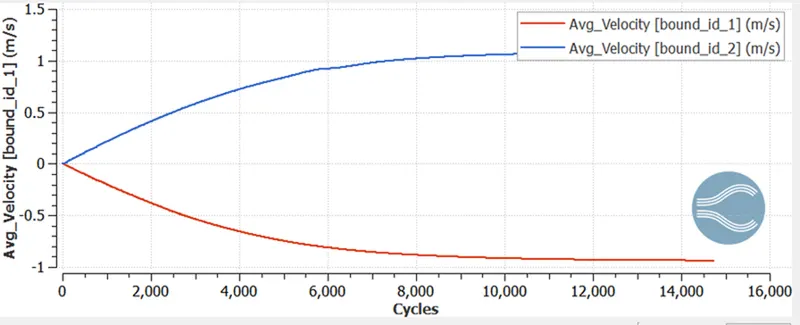
- In the above velocity plot, we easily observe that at the inlet velocity is gradually decreases due to increase in pressure at inlet
- At the outlet, we observe that the velocity is gradually increasing due decrease in pressure.
- At inlet the velocity is decreased and reaches to -1 m/s and at the outlet the velocity is increased and reaches to 1 m/s.
- It occurs since the pressure is inversely proportional to the velocity.
- Pressure Plot
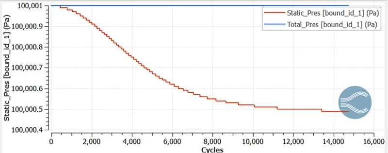
- At the inlet plot of pressure, we observe that initially total and static pressure is same which is 100,001Pa. And we also know that total pressure = static pressure+dynamic pressure and initially dynamic pressure is zero.
- As the cycles going on the static pressure is going to decrease due to increase in dynamic pressure.
- After 2000 cycles the static pressure is going to decrease rapidly due to fastly movement of fluid.
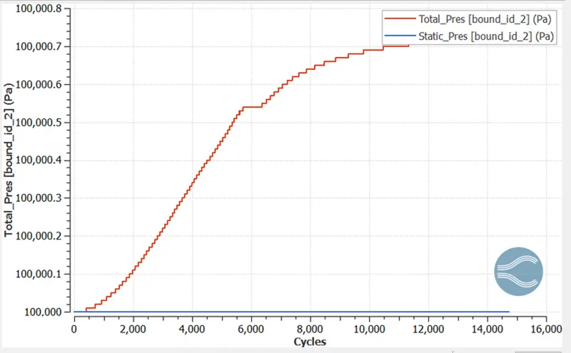
- Finally at the outlet the static pressure reaches to 100,000 Pa and the value of the total pressure is increases due to increase in dynamic pressure.
- Mass flow Rate Plot
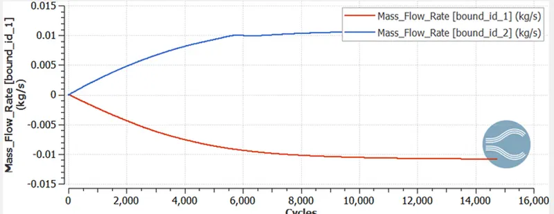
- Mass flow rate is defined as the mass of substance which passes per unit time.
- Here the mass flow rate at the inlet is decreased due to high pressure and low velocity and after 6000 cycles the mass flow rate is gradually decreases.
- Then Finally at the inlet the value of the mass flow rate is -0.01 (kg/s) and at the outlet the value of mass flow rate is 0.01 (kg/s).
- Total Cell Count
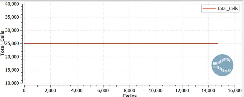
- Above graph shows the total cell count of channel flow case.
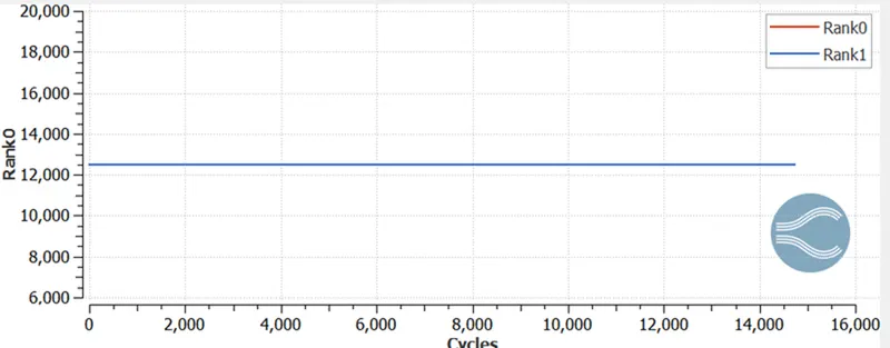
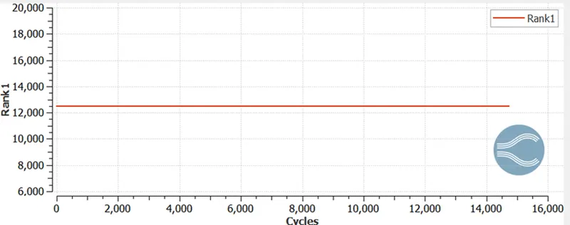
- Since i have used the 2 processors and the total cell count is 25000.
- Rank-0
- Rank-1
- For Mesh size 1.5e-04
- Velocity Plot
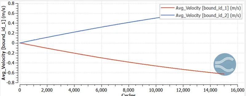
- In the above velocity plot, we easily observe that at the inlet velocity is gradually decreases due to increase in pressure at inlet.
- At the outlet, we observe that the velocity is gradually increase due decrease in pressure.
- At inlet the velocity is decreased and reaches to -0.7 m/s and at the outlet the velocity is increased and reaches to 0.7 m/s.
- It occurs since the pressure is inversely proportional to the velocity.
- Pressure Plot
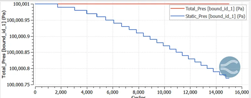
- At the inlet plot of pressure, we observe that initially total and static pressure is same which is 100,001Pa. And we also know that total pressure = static pressure+dynamic pressure and initially dynamic pressure is zero.
- As the cycles going on the static pressure is going to decrease due to increase in dynamic pressure.
- After 2000 cycles the static pressure is going to decrease rapidly due to fastly movement of fluid.
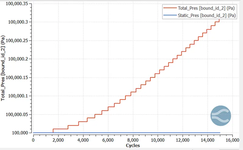
- Finally at the outlet the static pressure reaches to 100,000 Pa and the value of the total pressure is increases due to increase in dynamic pressure.
- Mass Flow Rate Plot
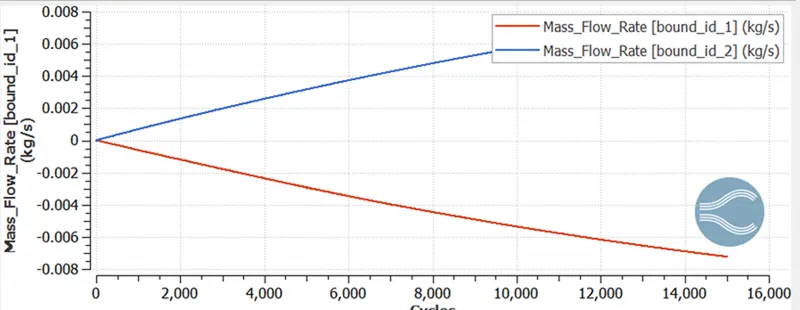
- Mass flow rate is defined as the mass of substance which passes per unit time.
- Here the mass flow rate at the inlet is decreased due to high pressure and low velocity and after 6000 cycles the mass flow rate is gradually decreases.
- Then Finally at the inlet the value of the mass flow rate is -0.007 (kg/s) and at the outlet the value of mass flow rate is 0.007 (kg/s).
- Total Cells
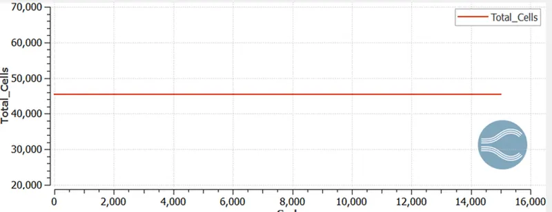
- Above graph shows the total cell count of channel flow case.
- Since i have used the 2 processors and the total cell count is 50,000.
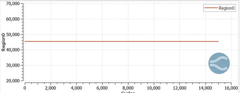
- Region-0
- For Mesh size 1e-04
- Velocity Plot
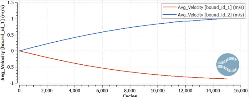
- In the above velocity plot, we easily observe that at the inlet velocity is gradually decreases due to increase in pressure at inlet
- At the outlet, we observe that the velocity is gradually increasing due decrease in pressure.
- At inlet the velocity is decreased and reaches to -1 m/s and at the outlet the velocity is increased and reaches to 1 m/s.
- It occurs since the pressure is inversely proportional to the velocity.
- Pressure Plot
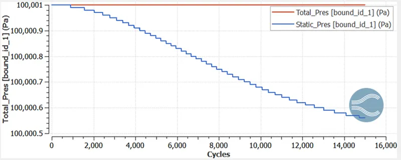
- At the inlet plot of pressure, we observe that initially total and static pressure is same which is 100,001Pa. And we also know that total pressure = static pressure+dynamic pressure and initially dynamic pressure is zero.
- As the cycles going on the static pressure is going to decrease due to increase in dynamic pressure.
- After 2000 cycles the static pressure is going to decrease rapidly due to fastly movement of fluid.
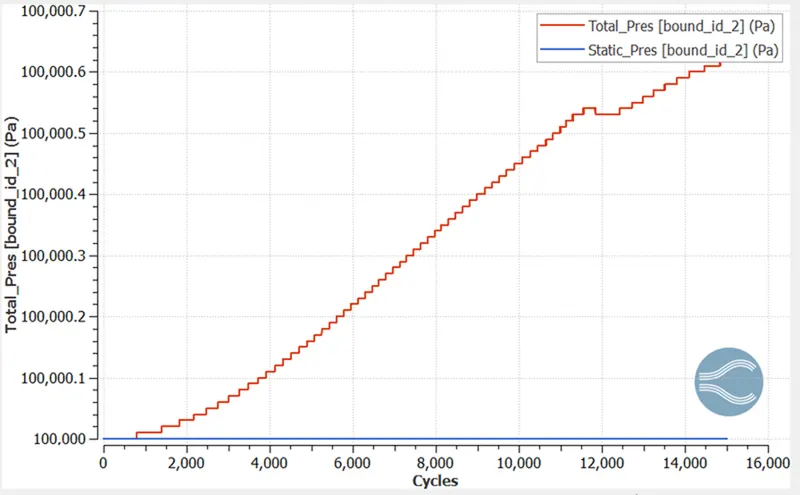
- Finally at the outlet the static pressure reaches to 100,000 Pa and the value of the total pressure is increases due to increase in dynamic pressure.
- Mass Flow Rate Plot
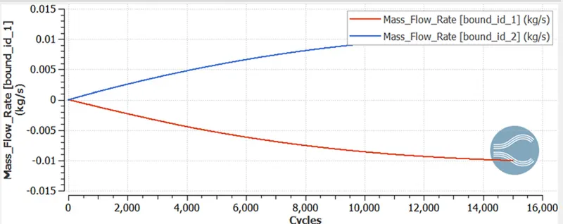
- Mass flow rate is defined as the mass of substance which passes per unit time.
- Here the mass flow rate at the inlet is decreased due to high pressure and low velocity and after 6000 cycles the mass flow rate is gradually decreases.
- Then Finally at the inlet the value of the mass flow rate is -0.01 (kg/s) and at the outlet the value of mass flow rate is 0.01 (kg/s).
- Total Cells
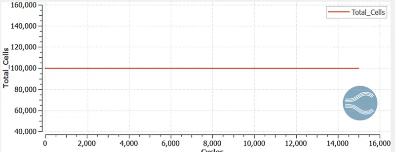
- Above graph shows the total cell count of channel flow case.
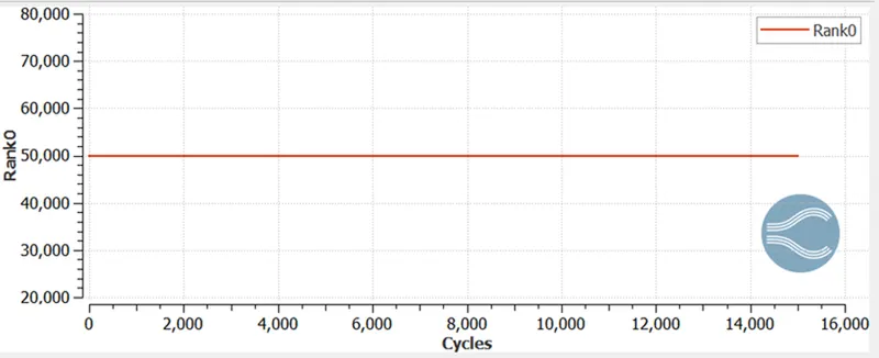
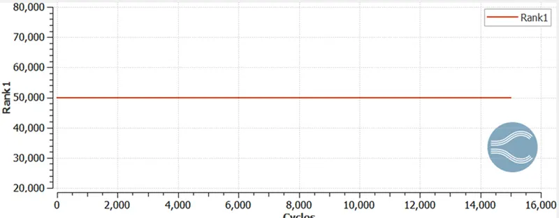
- Since i have used the 2 processors and the total cell count is 100,000.
- Rank-0
- Rank-1
Animation videos
Solution animation of mesh 2e-04
Solution animation of mesh 1.5e-04
Solution animation of mesh 1e-04
Conclusion:
- In this challenge, we simulate the 2D channel flow case using the converge.
- We run this case for three dufferent meshes. As the mesh gets fine, we got the more smooth results.
Channel Flow Simulation using Converge Software
Aim:
The main objective of this challenge is to simulate the simple 2D channel flow in converge CFD software. The simulation is done using three different meshes and compared the plots of velocity, pressure, total cell count and mass flow rate in all the meshes.
Geometry Preparation:
- First of all open the converge and launch the new project.
- Then in the Geometry box click on create then click on shape and then click on Box. After that enter the dimension of the channel case and then click on create.
- 3D view of the geometry.
- To create a boundary surface make sure that cursor picked the triangle.
- Then select the boundary, in the flag tab, click + to add the boundaries.
- Add the boundaries by clicking create multiple boubdaries to create all boundaries at a once and name them like inlet, outlet, top and bottom walls, front 2D and back 2D by selecting the respective triangles and click.
- Then click Nomal Toggle option and click any one of the triangle which shows the normal that is opposite to the direction of fluid flow and click Apply.
- Then click on options and under the tab of Visibility, click Geometry Bounding box to create boundary line across geometry.
- To ensure that the geometry is clean, click Diagnosis tab and click on Find.
- All the parameters that got checked shows the green colour tick mark.
Case-setup
- In order to begin the case-setup, click on the case-setup and click begin case-setup and click Time based, since it is not a crank angle based like IC engines or Pumps but a steady-state channel flow setup.
- Then click on Materials, uncheck the Reaction Mechanism since there is no chemical reaction takes place and select Air to be predefined mixtures.
- Since there is no role of turbulence here, click Physical Models and uncheck the Turbulence Modelling.
- Then open the Gas simulation and Global transport parameters and retain the default setting.
- Then click on Species and add the N2 and O2.
- Then click on the Run Parameter under the Simulation Parameter and choose the Steady state solver under the solver tab and then choose the Full Hydrodynmic under the simulation mode. And then choose the Compressible under the Gas flow solver.
- In the Miscellaneous tab, check the steady state monitor and uncheck the use shared memory because of we are running a steady state simulation flow here.
- At the inlet boundary we specify the inlet pressure 100001 Pa and select the predefined mixture as a Air which contains N2 as a 77% and O2 as 23%. And select the temperature to be specified of 300K.
- At the outlet boundary, we specify the 100000 Pa pressure.
- At the top and bottom walls, we are taken the no-slip condition.
- At the front and back boundary, we are taking the boundary type as a Two_D. To run a two dimensional simulation in converge, use the TWO-D boundary type. The TWO-D boundary is available only for non-moving and non-spray cases. To set up a two-dimensional case in CONVERGE, create a three-dimensional surface
including two identical, parallel boundaries and set their boundary type to TWO_D. Note that the normal vectors of the corresponding TWO_D boundaries must be in the z direction (positive or negative). Thus, the two-dimensional flow occurs in the xy plane. Ensure that in the surface geometry, no vertices exist in the thickness between the parallel TWO_D boundaries. - Then click on the Steady-state monitor, click add config. And click Add to add the variables that needs to be monitored.
- The monitor start display is a parameter that ensures that the simulaion runs for a certain number of cycles befoe the variable can be monitored. This is especially useful in transient simulations when you want the solution to run for a particular amount of time before checking for convergence, if the steady state results are also reuired.
- Sample size denotes the number of cycles or seconds over which the variable is checked to see if the solution has converged. The solution is said to be converge when the average change over multiples iterations is less than the tolerance value. The tolerance value can be changed based on the problem and level of accuracy required.
- In the simulation time parameter do the following changes.
- In Regions and Initializations, click Add as Region 0 and set pressure as 100000 Pa since the flow should not reversed and click Air as its species.
- Then in the grid control, the mesh size that want to be created is in meters.
- Then in the post variable selection, click on species/passive, check the mass fraction and add the N2 and O2.
- For Output files, Time inter for writing 3D output files is 100 cycles which is the time interval between the one and another output file that get dumped in output files successively and the maximum no. of restart files that saved is 3 which is a factor of safety and click ok.
- Now when we click on validate all options for validating, we got the errors.
- To Resolve these errors, we go to Regions and initializations and rename the region 0 to Voulmetric region user defined and then go Boundary to assign this region to all the boundaries we have ceated since the error is not assigning the region for those.
- And then click on validate all again and there will be no errors and the validation has been successfully complete.
- At the end all the inputs files have to be exported:
File -->Export-->Export input files
Mesh for the size 2e-04:
Mesh for the size 1.5e-04:
Mesh for the size 1e-04:
Analyzing the plots in Converge CFD
- For Mesh size 2e-04
Velocity Plot
- In the above velocity plot, we easily observe that at the inlet velocity is gradually decreases due to increase in pressure at inlet
- At the outlet, we observe that the velocity is gradually increasing due decrease in pressure.
- At inlet the velocity is decreased and reaches to -1 m/s and at the outlet the velocity is increased and reaches to 1 m/s.
- It occurs since the pressure is inversely proportional to the velocity.
- Pressure Plot
- At the inlet plot of pressure, we observe that initially total and static pressure is same which is 100,001Pa. And we also know that total pressure = static pressure+dynamic pressure and initially dynamic pressure is zero.
- As the cycles going on the static pressure is going to decrease due to increase in dynamic pressure.
- After 2000 cycles the static pressure is going to decrease rapidly due to fastly movement of fluid.
- Finally at the outlet the static pressure reaches to 100,000 Pa and the value of the total pressure is increases due to increase in dynamic pressure.
- Mass flow Rate Plot
- Mass flow rate is defined as the mass of substance which passes per unit time.
- Here the mass flow rate at the inlet is decreased due to high pressure and low velocity and after 6000 cycles the mass flow rate is gradually decreases.
- Then Finally at the inlet the value of the mass flow rate is -0.01 (kg/s) and at the outlet the value of mass flow rate is 0.01 (kg/s).
- Total Cell Count
- Above graph shows the total cell count of channel flow case.
- Since i have used the 2 processors and the total cell count is 25000.
- Rank-0
- Rank-1
- For Mesh size 1.5e-04
- Velocity Plot
- In the above velocity plot, we easily observe that at the inlet velocity is gradually decreases due to increase in pressure at inlet.
- At the outlet, we observe that the velocity is gradually increase due decrease in pressure.
- At inlet the velocity is decreased and reaches to -0.7 m/s and at the outlet the velocity is increased and reaches to 0.7 m/s.
- It occurs since the pressure is inversely proportional to the velocity.
- Pressure Plot
- At the inlet plot of pressure, we observe that initially total and static pressure is same which is 100,001Pa. And we also know that total pressure = static pressure+dynamic pressure and initially dynamic pressure is zero.
- As the cycles going on the static pressure is going to decrease due to increase in dynamic pressure.
- After 2000 cycles the static pressure is going to decrease rapidly due to fastly movement of fluid.
- Finally at the outlet the static pressure reaches to 100,000 Pa and the value of the total pressure is increases due to increase in dynamic pressure.
- Mass Flow Rate Plot
- Mass flow rate is defined as the mass of substance which passes per unit time.
- Here the mass flow rate at the inlet is decreased due to high pressure and low velocity and after 6000 cycles the mass flow rate is gradually decreases.
- Then Finally at the inlet the value of the mass flow rate is -0.007 (kg/s) and at the outlet the value of mass flow rate is 0.007 (kg/s).
- Total Cells
- Above graph shows the total cell count of channel flow case.
- Since i have used the 2 processors and the total cell count is 50,000.
- Region-0
- For Mesh size 1e-04
- Velocity Plot
- In the above velocity plot, we easily observe that at the inlet velocity is gradually decreases due to increase in pressure at inlet
- At the outlet, we observe that the velocity is gradually increasing due decrease in pressure.
- At inlet the velocity is decreased and reaches to -1 m/s and at the outlet the velocity is increased and reaches to 1 m/s.
- It occurs since the pressure is inversely proportional to the velocity.
- Pressure Plot
- At the inlet plot of pressure, we observe that initially total and static pressure is same which is 100,001Pa. And we also know that total pressure = static pressure+dynamic pressure and initially dynamic pressure is zero.
- As the cycles going on the static pressure is going to decrease due to increase in dynamic pressure.
- After 2000 cycles the static pressure is going to decrease rapidly due to fastly movement of fluid.
- Finally at the outlet the static pressure reaches to 100,000 Pa and the value of the total pressure is increases due to increase in dynamic pressure.
- Mass Flow Rate Plot
- Mass flow rate is defined as the mass of substance which passes per unit time.
- Here the mass flow rate at the inlet is decreased due to high pressure and low velocity and after 6000 cycles the mass flow rate is gradually decreases.
- Then Finally at the inlet the value of the mass flow rate is -0.01 (kg/s) and at the outlet the value of mass flow rate is 0.01 (kg/s).
- Total Cells
- Above graph shows the total cell count of channel flow case.
- Since i have used the 2 processors and the total cell count is 100,000.
- Rank-0
- Rank-1
Animation videos
Solution animation of mesh 2e-04
Solution animation of mesh 1.5e-04
Solution animation of mesh 1e-04
Conclusion:
- In this challenge, we simulate the 2D channel flow case using the converge.
- We run this case for three dufferent meshes. As the mesh gets fine, we got the more smooth results.