Week 4.1: Project - Steady state simulation of flow over a throttle body

Objective: To simulate (Steady state) the flow of fluid over the throttle body in a converge studio and post process the results.

1. Show the pressure and velocity contours.
2. Show the mesh (surface with edges).
3. Show the plots for pressure, velocity, mass flow rate and total cell count.

Basic of throttle valve:

Defnition of throttle valve

A valve designed to regulate the supply of a fluid (as steam or gas and air) to an engine and operated by a handwheel, a lever, or automatically by a governor. Especially : the valve in an internal-combustion engine incorporated in or just outside the carburetor and controlling the volume of vaporized fuel charge delivered to the cylinders.

Introduction:

A throttle is the mechanism by which fluid flow is managed by constriction or obstruction.

An engine's power can be increased or decreased by the restriction of inlet gases (by the use of a throttle), but usually decreased. The term throttle has come to refer, informally, to any mechanism by which the power or speed of an engine is regulated, such as a car's accelerator pedal. What is often termed a throttle (in an aviation context) is also called a thrust lever, particularly for jet engine powered aircraft. For a steam locomotive, the valve which controls the steam is known as the regulator.

In an internal combustion engine, the throttle is a means of controlling an engine's power by regulating the amount of fuel or air entering the engine. In a motor vehicle the control used by the driver to regulate power is sometimes called the throttle, accelerator, or gas pedal. For a gasoline engine, the throttle most commonly regulates the amount of air and fuel allowed to enter the engine. Recently, for a GDI engine, the throttle regulates the amount of air allowed to enter the engine. The throttle of a diesel, when present, regulates the air flow into the engine.

To regulate the power output from an engine there have to be some restriction of how much fuel - air mixture that reaches the cylinders. One way to do this is to use some kind of valve that restricts the air, fuel is then regulated to get the correct fuel - air mixture. The most common valve is of butterfly type and is used in almost every car engine manufactured today, the valve is sketched in the below figure

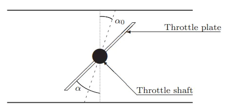
Most of the spark-ignition internal combustion engines operate with a stoichiometric air-gasoline ratio since it enables the catalyst to control emissions level. To control engine power, a throttle valve is used. The objective is to control air and consequently gasoline mass flow.

Valves that are utilized as fluid control devices are typically “throttling valves".

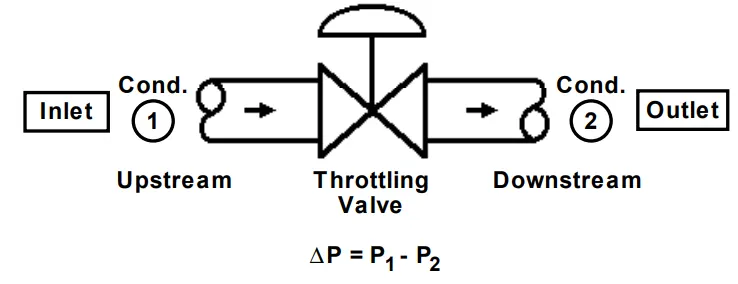
Such valves experience internal velocity and internal pressure gradients (both positive and negative) that conclude with a permanent pressure loss (∆P) from the inlet pipe-to-outlet pipe connections.

Geometry preparation:

• Open the new project and load the stl file of geometry.

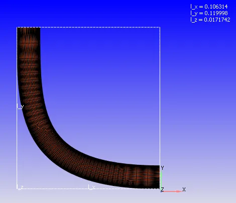
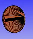
• Add the boundaries by clicking create multiple boubdaries to create all boundaries at a once and name them like Elbow_wall, Throttle_valve, top, inlet and outlet by selecting the respective triangles.

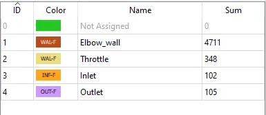
• Then click Normal Toggle option and click any one of the triangle which shows the normal that is opposite to the direction of fluid flow and click Apply.
• To ensure that the geometry is clean, click Diagnosis tab and click on Find.
• All the parameters that got checked shows the green colour tick mark.
• Case-setup
• In order to begin the case-setup, click on the case-setup and click begin case-setup and click Time based, since it is not a crank angle based like IC engines or Pumps but a steady-state channel flow setup.
• Then click on Materials and select Air to be predefined mixtures.
• Then open the Gas simulation and Global transport parameters and retain the default setting. And also retain the same setting for the species and Reaction mechanism.
• Then click on the Run Parameter under the Simulation Parameter and choose the Steady state solver under the solver tab and then choose the Full Hydrodynmic under the simulation mode. And then choose the Compressible under the Gas flow solver.
• In the Miscellaneous tab, check the steady state monitor and uncheck the use shared memory because of we are running a steady state simulation flow here.
• Then click on the Steady-state monitor, click add config. And click Add to add the variables that needs to be monitored.

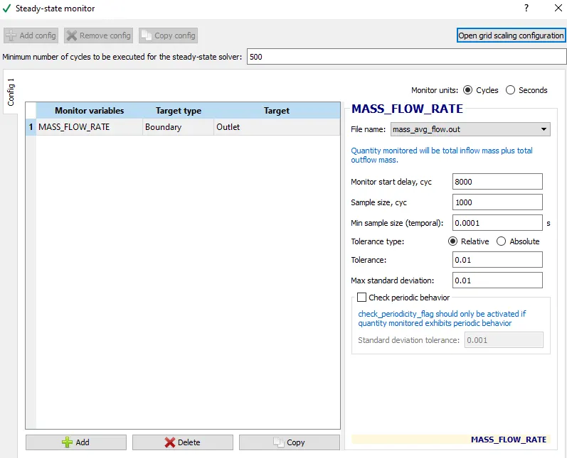
• The monitor start display is a parameter that ensures that the simulaion runs for a certain number of cycles before the variable can be monitored. This is especially useful in transient simulations when you want the solution to run for a particular amount of time before checking for convergence, if the steady state results are also required.
• Sample size denotes the number of cycles or seconds over which the variable is checked to see if the solution has converged. The solution is said to be converge when the average change over multiples iterations is less than the tolerance value. The tolerance value can be changed based on the problem and level of accuracy required.
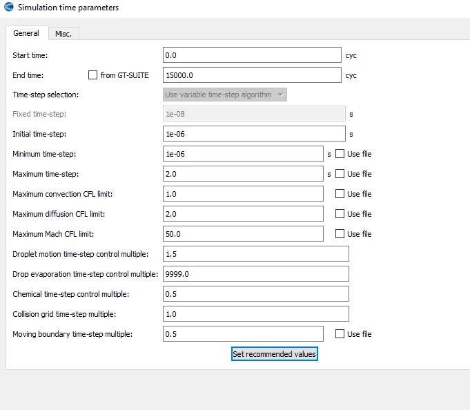
• In the simulation time parameter do the following changes.

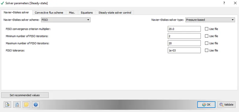
• In the solver time parameter, we only choose the pressure based solver and retain the remaining setting.

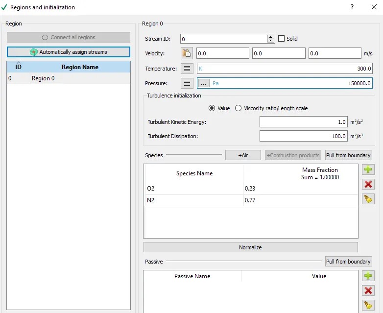
• At the inlet boundary we specify the inlet pressure 150000 Pa and select the predefined mixture as a Air which contains N2 as a 77% and O2 as 23%. And select the temperature to be specified of 300K.

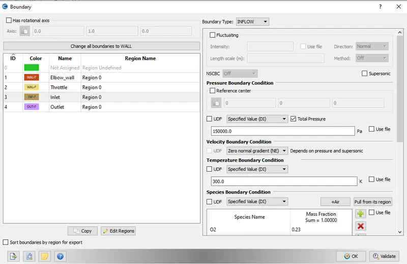
• At the outlet boundary, we specify the 100000 Pa pressure.

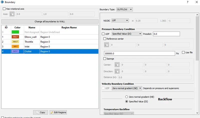
• At the Elbow and Throttle valve , we are taken the wall boundary condition.

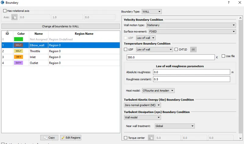
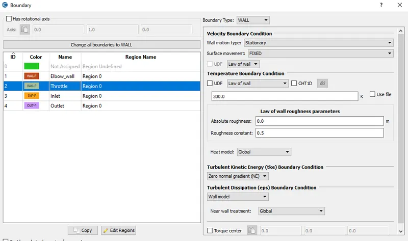
• In Regions and Initializations, click Add as Region 0.

• Goto Physical Models and check the Turbulence Modelling and choose the RNG/k-epsilon model.
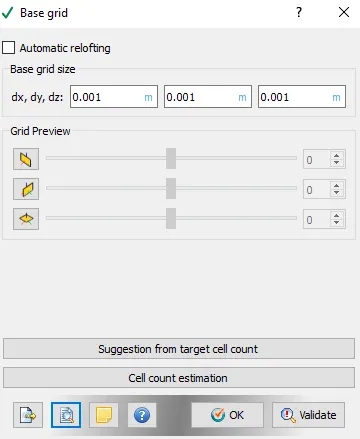
• Then in the grid control, the mesh size that want to be created is in meters.
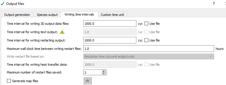
• For Output files, Time inter for writing 3D output files is 100 cycles which is the time interval between the one and another output file that get dumped in output files successively and the maximum no. of restart files that saved is 3 which is a factor of safety and click ok.

• Now when we click on validate all options for validating, we got the errors.
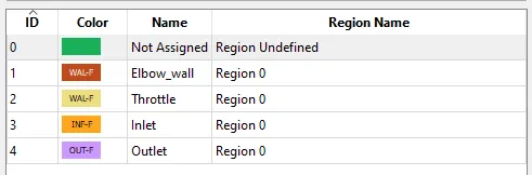
• To Resolve these errors, we go to Regions and initializations and rename the region 0 to Voulmetric region user defined and then go Boundary to assign this region to all the boundaries we have ceated since the error is not assigning the region for those.

• And then click on validate all again and there will be no errors and the validation has been successfully complete.
• At the end all the inputs files have to be exported:

File -->Export-->Export input files

Choice of grid scale in converge

Use fixed embedding to refine the grid at specific locations in the domain where a finer resolution is critical to the accuracy of the solution. For example, when simulating sprays, you can add an area of fixed embedding by the nozzle to resolve the complex flow behavior. Fixed embedding allows the rest of the grid to remain coarse to minimize simulation time. For each fixed embedding, you must specify an embedding scale that indicates how CONVERGE will refine the grid in that location. The embedding > embed_scale parameter in embedded.in, which must be a positive integer, scales the base grid sizes according to

`embed = frac{base grid}{2^(embed scal}`

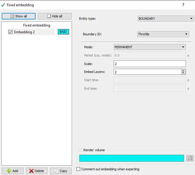
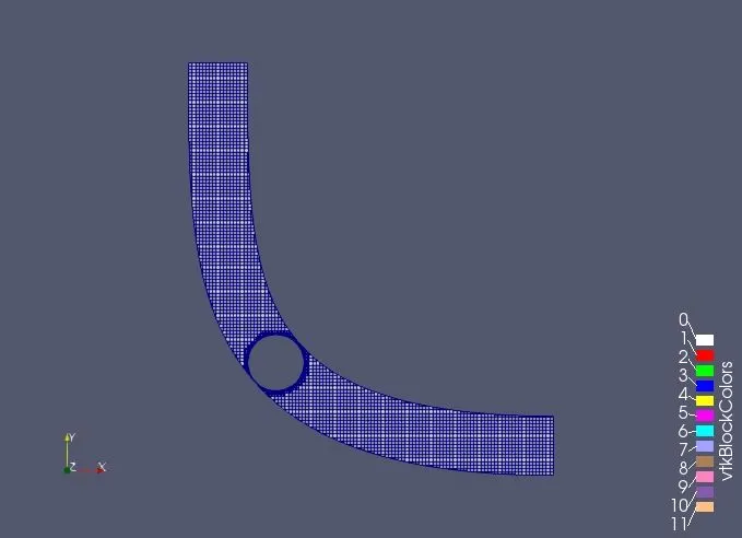
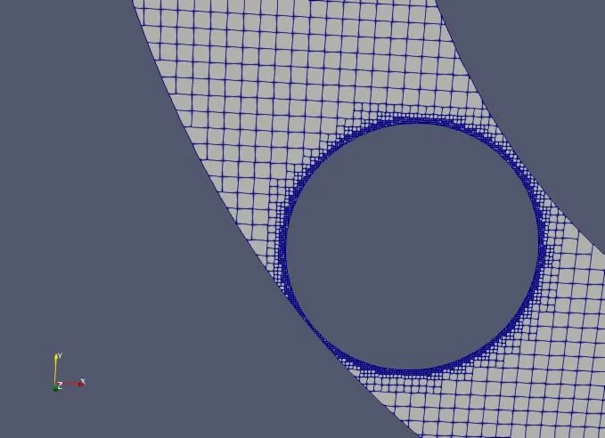
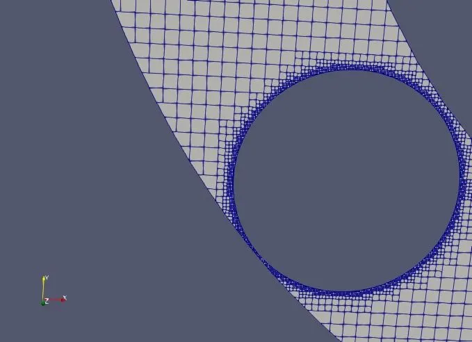
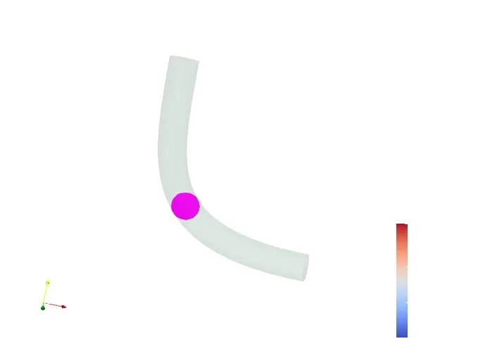
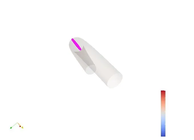
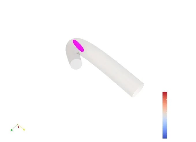
The mesh was refined locally near the throttle(empty circle) using fixed embedding to obtain more accurate results.

Analyzing the plots in Converge CFD

Mass flow rate:

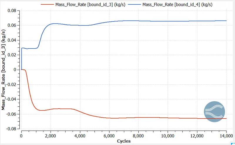
Bound_id_3 = inlet boundary, Bound_id_4 = Outlet boundary

• Mass flow rate is defined as the mass of substance which passes per unit time.
• Here the mass flow rate at the inlet is decreased due to high pressure and low velocity and after 2000 cycles the mass flow rate is gradually decreases.
• Then Finally at the inlet the value of the mass flow rate is -0.065 (kg/s) and at the outlet the value of mass flow rate is 0.065 (kg/s).
• At the inlet negative sign shows that the mass is going to inside and the outlet positive sign shows that the mass is going to outside.

Velocity plot

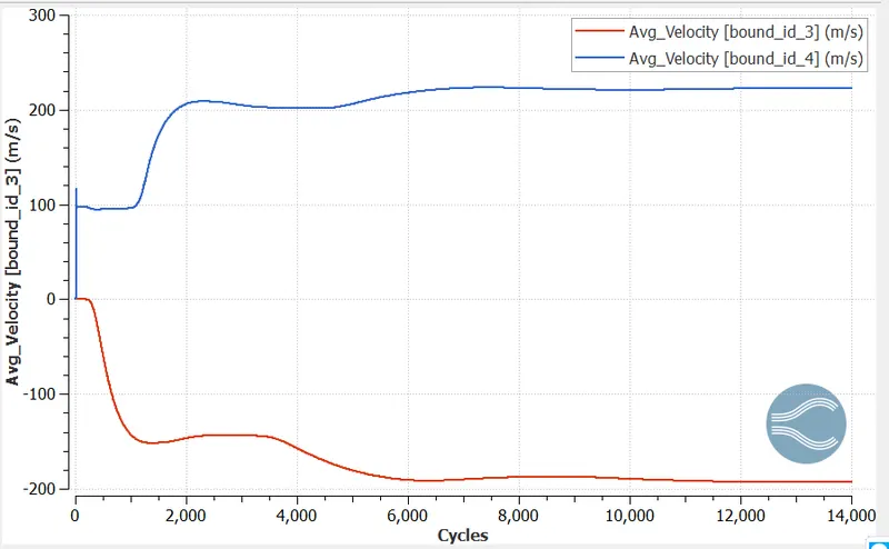
• In the above velocity plot, we easily observe that at the inlet velocity is gradually decreases due to increase in pressure at inlet
• At the outlet, we observe that the velocity is gradually increasing due decrease in pressure.
• At inlet the velocity is decreased and reaches to -199 m/s and at the outlet the velocity is increased and reaches to 220 m/s.
• It occurs since the pressure is inversely proportional to the velocity.

Pressure Plot:

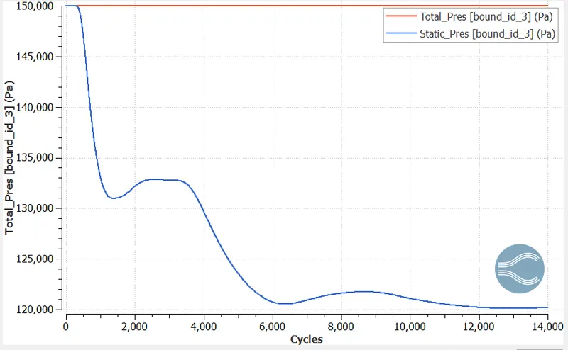
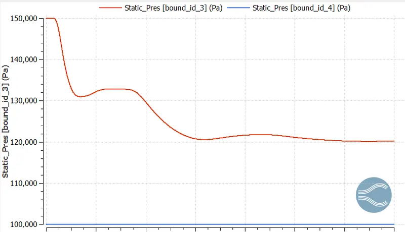
• At the inlet plot of pressure, we observe that initially total and static pressure is same which is 150,000 Pa. And we also know that total pressure = static pressure+dynamic pressure and initially dynamic pressure is zero.
• As the cycles going on the static pressure is going to decrease due to increase in dynamic pressure.
• After 1500 cycles the static pressure is going to decrease rapidly due to fastly movement of fluid.

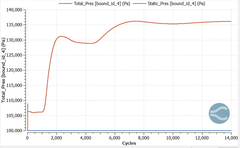
• Finally at the outlet the static pressure reaches to 136,000 Pa and the value of the total pressure is increases due to increase in dynamic pressure.

Total Pressure

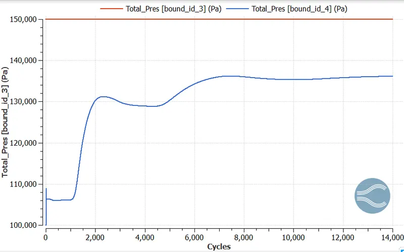
Static pressure

Total cell count

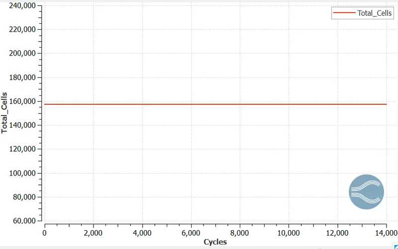
• Above graph shows the total cell count of throttle valve case.
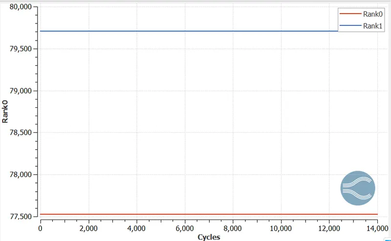
• Since i have used the 2 processors and the total cell count is 160,000.

Pressure Contours

Observation from plot

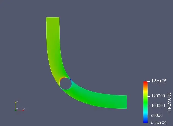
In the above plot we can easily observe the two regions which we can see

• Red region shows the high pressure which is between 1.4 to 1.5 bar.
• And blue region shows the low pressure. The pressure drop because the flow is constricted.

Pressure contours plot on the throttle:

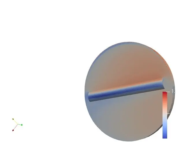
• On the throttle, we also observe the two region which is red and blue. Red colour shows the high pressure region and blue colour shows the low pressure region. In high pressure region fluid impose the pressure on the throttle as it flows over the throttle body.
• And the low pressure region(blue region) is due to the flow separation happening near the axis of rotation of the throttle.

Velocity Contours

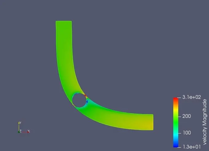
Observation from plot

In the above plot we can easily observe the three regions which we can see

• Top left blue colour region shows that the velocity decreases as it is near about about the throttle.
• Red region shows the high velocity which is approximately 310 m/s. This is the narrow path where the fluid passses and that's why velocity is increases.
• And bottom right blue region shows the recirculation region. Flow separation is also occuring here, eddies are formed here and velocity drops as low as 20 m/s.

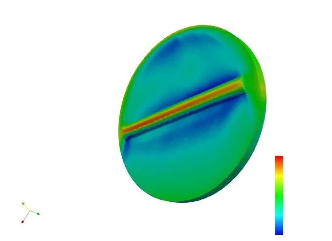
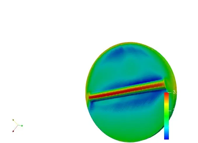
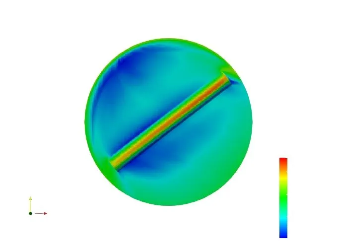
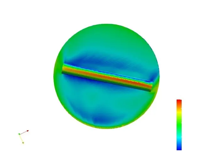
On the throttle, we also observe the two region which is red and blue. Red colour shows the high velocity region and blue colour shows the low velocity region.

Velocity animation:

Pressure animation: