Week 4.1 - Genetic Algorithm

AIM:

• A program in matlab to simulate the to understand the concept of genetic algorithm by referring to varius sources.

CONCEPT:

• Genetic Algorithm (GA) is a search-based optimization technique based on the principles of Genetics and Natural Selection. It is frequently used to find optimal or near-optimal solutions to difficult problems which otherwise would take a lifetime to solve.
• It is frequently used to solve optimization problems, in research, and in machine learning.
• This section introduces the basic terminology required to understand GAs.
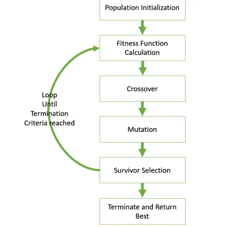
• Also, a generic structure of GAs is presented in both pseudo-code and graphical forms.
• We start with an initial population (which may be generated at random or seeded by other heuristics), select parents from this population for mating.
• Apply crossover and mutation operators on the parents to generate new off-springs. And finally these off-springs replace the existing individuals in the population and the process repeats.
• Population is a subset of solutions in the current generation. It can also be defined as a set of chromosomes. There are several things to be kept in mind when dealing with GA population −

• The diversity of the population should be maintained otherwise it might lead to premature convergence.

• The population size should not be kept very large as it can cause a GA to slow down, while a smaller population might not be enough for a good mating pool. Therefore, an optimal population size needs to be decided by trial and error.

OBJECTIVE:

• The main objective of the program is to create a program to calculate the concept of genetic algorithm with the help of MATLAB.

BODY OF THE CONTENT:

• SOFTWARE USED - MATLAB.

{MAIN CODING OF THE PROGRAM}

% Genetic_Algorithm
clear all
close all
clc

%define the space for objective function

x = linspace(0,0.6,180);

y = linspace(0,0.6,180);

%evaluation of objective funtion

for i = 1:length(x)
    for j = 1:length(y)
        inputs(1)=x(i);
        inputs(2)=y(j);
        f(i,j) = stalagmite(inputs);
    end
end



for k = 1:100

    [inputs,fopt(k)]= ga(@stalagmite,2,[],[],[],[],[0;0],[0.4;0.4]);
    xopt(k) = inputs(1);
    yopt(k) = inputs(2);
    
end

figure(1);
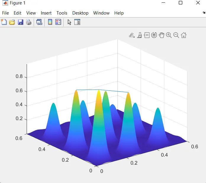
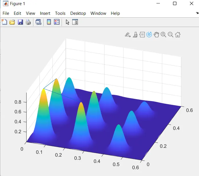
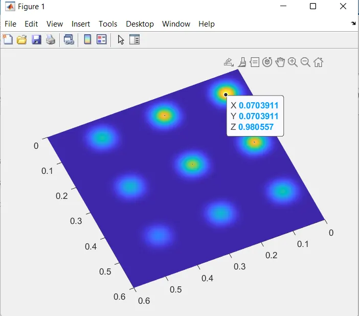
surfc(x,y,-f)
shading interp
hold on
plot3(xopt,yopt,-fopt)



function [f]= stalagmite(input)
x = input(1);
y = input(2);
fx1 = (sin((5.1*pi)*input(1)+0.5))^6;
fy1 = (sin((5.1*pi)*input(2)+0.5))^6;

fx2 = exp(-4*log(2)*((input(1) - 0.0667)^2)/0.64);
fy2 = exp(-4*log(2)*((input(2) - 0.0667)^2)/0.64);
f = -(fx1*fx2*fy1*fy2);
end

CODING EXPLATION:

• First few lines are the Basic commands of the coding.
• clear all command is used to clear all the variables from the current work space.
• close all command is used to close all figures whose handles are vissible.
• Defining the user defined inputs.
• x and y are the inputs of the function respectively.
• Using for loop function to multiple values of the arrays.
• perform the loop variables properly inside the for loop command.
• using the shading interp comand is used to shade the full pill of the graph.
• ploting is used to plot the three points of x,y,f.

OUTPUT RESULTS:

CONCLUTION:

• As a conclution of this program tought me a basic ideas about to mergh a function in main program.
• In the programing point i learnt a bit more clear about the FOR LOOP function.
• Eventhough i am new to programing the tutorial video was very clear and helped me a lot to understand this functioning.